
5
GHIDRA DATA DISPLAYS

At this point, you should have some confidence creating projects, loading binaries into projects, and initiating auto analysis. Once Ghidra’s initial analysis phase is complete, it is time for you to take control. As discussed in Chapter 4, when you launch Ghidra, your adventure starts in the Ghidra Project window. When you open a file within one of your projects, a second window opens. This is the Ghidra CodeBrowser, and it’s your home base for much of your SRE efforts. You’ve already used the CodeBrowser to auto analyze your file; now we’ll take a deeper dive into the CodeBrowser menu, windows, and basic options to increase your awareness of Ghidra’s capabilities and allow you to create an SRE analysis environment that is consistent with your personal workflow. Let’s begin with the principal Ghidra data displays.
CodeBrowser
You can open the CodeBrowser window by selecting Tools ▸ RunTool ▸ CodeBrowser from the Ghidra Project window. Although CodeBrowser is generally opened by selecting a file for analysis, we are opening an empty instance so that the functionality and configuration options can be demonstrated without specific file-related content influencing the display, as shown in Figure 5-1. In its default configuration, CodeBrowser has six subwindows. Before we get into the details associated with each of these displays, let’s spend a little time looking at the CodeBrowser menu and its associated functionality.
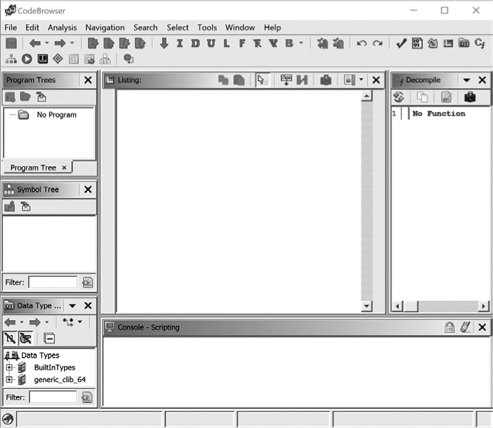
Figure 5-1: Unpopulated CodeBrowser window
At the top of the CodeBrowser window is the main menu with a toolbar immediately below. The toolbar provides one-click shortcuts to some of the most commonly used menu options. As we do not currently have a file loaded, we will focus on the menu options that are not associated with a loaded file in this section. Other menu actions will be demonstrated and explained in context with their applicability to the SRE process.
File Provides the basic functionality expected in most file manipulation menus, including options for Open/Close, Import/Export, Save, and Print. In addition, some options are specific to Ghidra, such as Tool options, which allow you to save and manipulate the CodeBrowser tool, and Parse C Source, which can aid in the decompilation process by extracting data type information from C header files. (See “Parsing C Header Files” on page 269.)
Edit Includes one command that is applicable outside individual subwindows: the Edit ▸ Tool Options command, which opens a new window that allows you to control parameters and options associated with the many tools available from the CodeBrowser. The options related to the console are shown in Figure 5-2. The Restore Defaults button (revert to default settings) is always available at the bottom right.

Figure 5-2: CodeBrowser Console edit options
Analysis Allows you to reanalyze a binary or selectively perform individual analysis tasks. The basic analysis options were introduced in “Analyzing Files with Ghidra” on page 48.
Navigation Facilitates navigation within files. This menu provides the basic keyboard functionality supported by many applications and adds special navigation options for binaries. While the menu provides one method for moving through a file, you will likely use toolbar options or shortcuts (listed at the right of each menu option) after you gain experience with the many options available for navigation.
Search Provides search capabilities for memory, program text, strings, address tables, direct references, instruction patterns, and much more. Basic searching functionality is introduced in “Searching” on page 114. More specialized search concepts are presented in context as part of the many examples in subsequent chapters.
Select Provides the capability to identify a portion of the file to consider for a specific task. Selections can be based on subroutines, functions, control flows, or simply by highlighting a desired portion of the file.
Tools Includes some interesting features that allow you to place additional SRE resources on your desktop. One of the most useful is the Processor Manual option, which brings up the processer manual associated with the current file. If you attempt to open a missing processor manual, you will be provided with a method to include the manual, as shown in Figure 5-3.
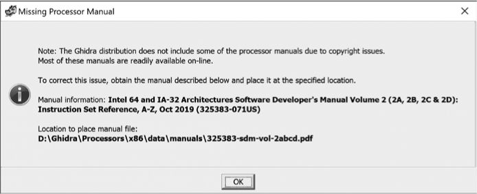
Figure 5-3: Missing Processor Manual message
Window Allows you to configure your Ghidra work environment for your workflow. We spend most of this chapter introducing and investigating the default Ghidra windows as well as some others that you will find helpful.
Help Provides rich, well-organized, and very detailed options. The Help window supports searching, different views, favorites, zooming in/out, as well as printing and page setup options.
CodeBrowser Windows
The expanded Window menu can be seen running down the center of Figure 5-4. By default, six of the available windows are opened when CodeBrowser is launched: Program Trees, Symbol Tree, Data Type Manager, Listing, Console, and Decompiler. The name of each window is displayed at the top left of the associated window. Each of these windows appears as an option on the Window menu, and some also have associated icons on the toolbar directly below the menu. (As an example, we’ve used arrows in Figure 5-4 to highlight the toolbar option and menu option for opening and accessing the Decompiler window.)
HOTKEYS AND BUTTONS AND BARS, OH MY!
Almost all commonly used actions within Ghidra have an associated menu item, hotkey, and toolbar button. If they don’t, you have the power to create them! The Ghidra toolbar is highly configurable, as is the mapping of hotkeys to menu actions. (See CodeBrowser Edit ▸ Tool Options ▸ Key Bindings or just hover over a command and press F4.) As if this wasn’t enough, Ghidra also offers good, context-sensitive menu actions in response to right mouse clicks. While these context-sensitive menus do not offer an exhaustive list of permissible actions at a given location, they do serve as good reminders for the most common actions you will be performing. This flexibility allows you to perform an action using the means most comfortable to you and to customize the environment as you discover how Ghidra can work for you.
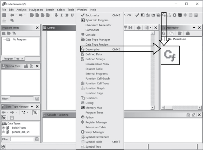
Figure 5-4: CodeBrowser window with options to display Decompiler window emphasized
Let’s dive into the six default windows to understand their fundamental importance in the SRE process.
WINDOW INSIDERS AND OUTSIDERS
As you begin exploring the various Ghidra windows, you will notice that, by default, some windows open within the CodeBrowser desktop and others open as new floating windows outside the CodeBrowser desktop. Let’s take a minute to talk about these “insiders” and “outsiders” in the context of the Ghidra environment.
The “outsider” windows float outside the CodeBrowser environment and may be connected or independent. These windows allow you to explore their contents side by side with CodeBrowser. Examples of these windows are Function Graph, Comments, and Memory Map.
Next, there are three distinct classes of “insider” windows:
- Windows that open by default in CodeBrowser (for example, Symbol Tree and Listing)
- Windows that are stacked with a default CodeBrowser window (for example, Bytes)
- Windows that create or share space with other CodeBrowser windows (for example, Equates and External Programs)
When you open a window that shares a space with another open window, it appears in front of the existing window. All windows sharing the same space are tabbed to allow rapid navigation between windows. If you want to view two windows that share a space simultaneously, you can click the title bar of the window and drag it outside the CodeBrowser window.
But be careful! Getting windows back into the CodeBrowser window is not as easy as moving them out. (See “Rearranging Windows” on page 242 for more details.)
WHERE’S MY WINDOW?
Ghidra has a lot of windows, and it can be challenging to keep track of where they are at any particular time. This becomes even more complicated as you open more windows and others disappear behind them in CodeBrowser or on your desktop. Ghidra has a unique feature to help you locate those missing windows. Clicking the associated toolbar icon or menu item will move the selected window to the front, but that might not be enough. If you continue clicking the toolbar icon for the window, your missing window will try to catch your attention by vibrating, changing font size or colors, zooming, spinning, and other exciting motions that are sure to catch your eye to help you find it. If you are bored, you can wave back.
The Listing Window
Also known as the Disassembly window, the Listing window will be your primary tool for viewing, manipulating, and analyzing Ghidra-generated disassemblies. The text display presents the entire disassembly listing of a program and provides the primary means for viewing the data regions of a binary.
The CodeBrowser display for ch5_example1.exe is shown in its default configuration in Figure 5-5. The margin to the left of the Listing window provides important information about the file as well as your location within the file. There is an additional marker area on the right side of the Listing window (immediately to the right of the vertical scroll bar) that also provides important information and navigational capabilities. The scroll bar indicates your location within the file and can be used for navigation. To the immediate right of the scroll bar are some informational displays, including bookmarks, that provide additional insight into the file.
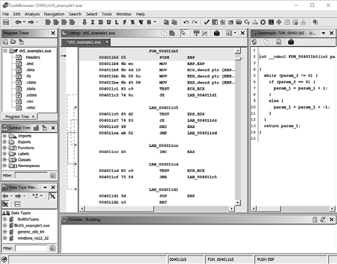
Figure 5-5: Default CodeBrowser window with ch5_example1.exe loaded
YOUR FAVORITE BARS
After a file is auto analyzed, you can use informational margin bars to help you navigate and further analyze the file. By default, only the Navigation bar is displayed. You can choose to add (or hide) the Overview bar and Entropy bar by using the Toggle Overview Margin tool button at the top right of the Listing window (see Figure 5-6). Regardless of which bars are displayed, a navigation marker to the left of all of the bars reminds you of where you are in the file. Left-clicking any location in any of the bars will move you to that location in the file and update the contents of the Listing window.
Now that you know how to control the appearance (and disappearance) of the bars, let’s investigate what each bar shows and how you might use it in your SRE process:
Navigation Marker area Allows you to move through the file, but it also has another very important function: if you right-click the Navigation Marker area, you will see the classes of markers and bookmarks that can be associated with your file. By selecting and deselecting marker types, you can control what is displayed in the Navigation bar. This allows you to easily move through particular types of markers (such as highlights).
Overview bar Provides you with important visual information about the contents of a file. The horizontal bands in the Overview bar represent color-coded regions of the program. While Ghidra provides default colors associated with common categories, such as functions, external references, data, and instructions, you can control the color scheme through the Edit ▸ Tool Options menu. By default, if you hover over a region, you can view detailed information about that region, including the region type and an associated address, if applicable.
Entropy bar Provides a unique Ghidra functionality: it “stereotypes” file content based on the file content around it. If there is very little variation within a region, it is assigned a low entropy value. If there is high degree of randomness, the corresponding entropy value is high. Hovering your mouse over a horizontal band in the Entropy bar will give you the entropy value (between 0.0 and 8.0), a type (for example, .text), as well as the associated address in the file. The highly configurable Entropy bar can be used to help determine the most likely content in the band. More information about this capability and the mathematics behind it can be discovered in the Ghidra Help menu.
Figure 5-6 provides a breakdown of tool buttons specific to the Listing window. In Figure 5-7, we have expanded and zoomed in on the Listing window to investigate what is shown. The disassembly is presented in linear fashion, with the leftmost column displaying virtual addresses by default.

Figure 5-6: Listing window tool buttons

Figure 5-7: Listing window with labeled example artifacts
Within the Listing window are several items that merit your attention. The gray band at the far left of the window is the margin marker. It is used to indicate your current location in the file and includes point markers and area markers, which are described in Ghidra Help. In this example, the current file location (004011b6) is indicated in the margin marker by the small black arrow.
The region immediately to the right of the margin marker is used to graphically depict nonlinear flow within a function.1 When the source or target address for a control flow instruction is visible in the Listing window, associated flow arrows appear. Solid arrows represent unconditional jumps, while dashed arrows represent conditional jumps. Hovering over a flow line opens a tool tip that displays the start and end address of the flow along with the flow type. When a jump (conditional or unconditional) transfers control to an earlier address in the program, it is often indicative of a loop. This is demonstrated in Figure 5-7 by the flow arrow from address 004011cf to 004011c5. You can easily navigate to the source or destination of any jump by double-clicking the associated flow arrow.
The declarations at the top of Figure 5-7 show Ghidra’s best estimate concerning the layout of the function’s stack frame.2 Ghidra computes the structure of a function’s stack frame (local variables) by performing detailed analysis of the behavior of the stack pointer and any stack frame pointer used within a function. Stack displays are discussed further in Chapter 6.
Listings generally have numerous data and code cross-references indicated by XREF, seen on the right side of Figure 5-7. A cross-reference is created anytime one location in the disassembly refers to another location in the disassembly. For example, an instruction at address A jumping to an instruction at address B would result in the creation of a cross-reference from A to B. Hovering over a reference address causes a reference pop-up to appear with the referencing location. The reference pop-up is in the same layout as the Listing window but has a yellow background (similar to a tool tip pop-up). The pop-up window allows you to view the content but does not allow you to follow the references. Cross-references are the subject of Chapter 9.
Creating Additional Disassembly Windows
If you ever find yourself wanting to view a listing of two functions simultaneously, all you need to do is open another disassembly window by using the Snapshot icon in the Listing toolbar (refer to Figure 5-6). The first disassembly window opened has the prefix Listing: before the filename. All subsequent disassembly windows are titled [Listing: <filename>] to indicate that they are disconnected from the primary display. The snapshots are disconnected so you can navigate freely through them without affecting other windows.
CONFIGURING LISTING WINDOWS
A disassembly listing may be decomposed into a number of component fields, including information such as a mnemonic field, an address field, and a comment field. The listings we have seen so far have been composed from a default set of fields that provide important information about the file. However, sometimes the default view does not provide the information you would like to see. Enter the Browser Field Formatter.
The Browser Field Formatter provides you the ability to customize over 30 fields to ensure you have ultimate control over the appearance of your Listing windows. You can activate the Browser Field Formatter by clicking the button in the Listing toolbar (refer to Figure 5-6). This opens a powerful submenu and layout editor, seen in Figure 5-8, at the top of the listing. The Browser Field Formatter allows you to control the appearance of address breaks, plate comments, functions, variables, instructions, data, structures, and arrays. Within each of these categories are fields that you can adjust, tune, and control to create the perfect listing format for you. We stick primarily with the default formats for listings, but you should explore the Browser Field Formatter to determine whether any options improve your understanding of the Listing window contents.

Figure 5-8: Listing window with Browser Field Formatter activated
Ghidra Function Graph View
While assembly listings are interesting and informative, the flow of the program might be easier to understand by viewing a graph-based display. You can open a Function Graph window associated with the CodeBrowser by choosing Window ▸ Function Graph or clicking the associated icon in the CodeBrowser toolbar. The Function Graph window corresponding to the function in Figure 5-7 is shown in Figure 5-9. Graph views are somewhat reminiscent of program flowcharts in that a function is broken into basic blocks so you can visualize the function’s control flow from one block to another.3
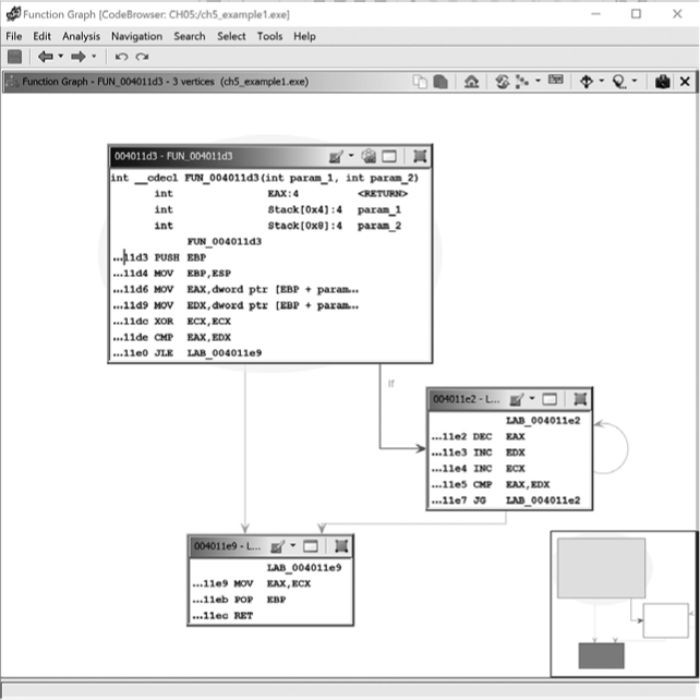
Figure 5-9: Graph view of listing from Figure 5-7
Onscreen, Ghidra uses different-colored arrows to distinguish various types of flows between the blocks of a function. In addition, the flows become animated as you mouse over them to indicate direction. Basic blocks that terminate with a conditional jump generate two possible flows: the Yes edge arrow (yes, the tested condition was met) is green by default, and the No edge arrow (no, the tested condition was not met) is red by default. Basic blocks that terminate with only one potential successor block use a Normal edge (blue by default) to point to the next block to be executed. You can click any arrow to see the associated transition from one block to another. Since the graph and listing tools are synchronized by default, your file location will generally remain consistent when switching between and navigating within the listing view and graph view. Exceptions are discussed in Chapter 10 as well as in Ghidra Help.
In graph mode, Ghidra displays one function at a time. Ghidra facilitates navigation around the graph by using traditional image interaction techniques such as pan and zoom. Large or complex functions may cause the graph to become extremely cluttered, making the graph difficult to navigate, which is where the Satellite View can help you. By default, the Satellite View is positioned at the bottom right of the graph window and can be a valuable aid to provide some situational awareness (see Figure 5-9).
SATELLITE NAVIGATION
The Satellite View always displays the complete block structure of the graph along with a highlighted frame that indicates the region of the graph currently being viewed in the disassembly window. Clicking any block in the Satellite View centers the graph around that block. The highlighted frame acts as a lens and can be dragged around the overview window to rapidly reposition the graph view to any location on the graph. In addition to providing a means to navigate the Function Graph window, this magical window has other powers that can work for or against you as you examine files.
This window consumes valuable space in your Function Graph window and can hide important blocks and contents just when you want to see them. There are two approaches to remedy this situation. You can right-click the Satellite View and uncheck the Dock Satellite View checkbox. This will move the Satellite View and its full functionality outside the Function Graph window. Rechecking the option at any time will move it back to its original location in the Function Graph window.
A second option is to hide the Satellite View, provided you don’t need to use it to navigate. This is another checkbox available in the right-click context menu. When you hide the Satellite View, a small icon will appear in the bottom right of the Function Graph window. Clicking this icon will restore the Satellite View.
When visible, the Satellite View can cause the primary view to behave more slowly than desired. Hiding the Satellite View can help to make it more responsive.
TOOLS MAKING CONNECTIONS
Tools can operate together or independently. We have seen how the Listing window and the Function Graph window share data and how events that occur in one window affect the other. If you select a particular block in the Function Graph window, the corresponding code will be highlighted in the Listing window. Conversely, navigating between functions in the Listing window will cause the Function Graph window to be updated. This is one of the many tool connections that happens automatically and is bidirectional. Ghidra also has capabilities for unidirectional connections as well as the ability to manually connect and disconnect tools using a producer/consumer model associated with tool events. In this book, we focus on the bidirectional automatic tool connections that Ghidra provides.
In addition to navigating with the Satellite View, you can manipulate the view within the Function Graph window in many ways to suit your needs:
Panning First, in addition to using the Satellite View to rapidly reposition the graph, you can reposition the graph by clicking and dragging the background to change the graph view.
Zooming You can zoom in and out using traditional keyboard methods such as CTRL/COMMAND, a mouse scroll, or associated key bindings. If you zoom out too far, you may pass the painting threshold, where the block contents are no longer displayed. Each block just becomes a colored rectangle. In some cases, particularly when working side by side with the Listing window, this might be advantageous, as it improves the speed at which the function graph can be rendered.
Rearranging blocks Individual blocks within the graph can be dragged to new positions by clicking the title bar for the desired block and dragging it to a new position. All links between blocks are preserved as you move the blocks. If at any point you find yourself wishing to revert to the default layout for your graph, you can do so by selecting the Refresh icon in the Function Graph toolbar.
Grouping and collapsing blocks Blocks can be grouped, either individually or together with other blocks, and collapsed to reduce the clutter in the display. Grouping causes a block to collapse. Collapsing blocks is an easy method to keep track of the blocks you have analyzed. You can collapse any block by choosing the Group icon in the far right of the block toolbar. If you choose this option with multiple blocks selected, they will be collapsed, and the list of associated blocks will be displayed in the stacked window. Some nuances are associated with forming/unforming groups as well as performing actions on the newly formed groups that are explained in Ghidra Help.
CUSTOMIZING YOUR GRAPH DISPLAY
To help you with your analysis, Ghidra provides a menu bar at the top of each node in the Function Graph display that allows you to control the display for that particular node. You can control background/text color for the node, jump to an XREF, view a full window listing of the graph node, and use grouping functionality to combine and collapse nodes. (Note that changing the background for a block in the Function Graph also changes the background in the Listing window.) Some of these features might be unnecessary if you are actively using the Listing window in conjunction with the Function Graph window, but the customization options may be helpful and are certainly worth investigating. These options are discussed further in Chapter 10.
As the graph-based display opens in a window external to CodeBrowser, you can view the two displays side by side. Because the windows have a connection, changing locations in one of the windows moves the location marker in the other window. While many users tend to prefer one view over the other to visualize program flow, you don’t have to choose only one. Also, keep in mind that your control over the graph and text views extends far beyond these examples. Additional Ghidra graphing capabilities are covered in Chapter 10, while more information on the manipulation of Ghidra’s view options is available in Ghidra Help.
For the next five chapters, we primarily focus on the listing display for examples, supplemented with the graph display in cases where it adds significant clarity. In Chapter 6 we will focus on understanding a Ghidra disassembly, and in Chapter 7, we cover the specifics of manipulating the listing display in order to clean up and annotate a disassembly.
MOVING AROUND
In addition to traditional means of navigating a file (up arrow, down arrow, page up, page down, and so on), Ghidra provides navigation tools specific to the SRE process. The icons in the Navigation toolbar (shown in Figure 5-10) make it easy to move through the program. Let’s meet the icons that serve the reverse engineer.
Figure 5-10: CodeBrowser Navigation toolbar
On the far left is the Direction icon. This arrow toggles between up and down and controls the direction for all of the other navigation icons. The next eight icons advance you through the various targets shown in Figure 5-11.
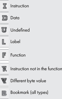
Figure 5-11: Navigation toolbar definitions
Rather than just advancing you to the next data in the listing, choosing the Data option skips over adjacent data and takes you to the start of the next nonadjacent data. Instruction and Undefined demonstrate the same behavior.
The drop-down arrow at the far right of the Navigation toolbar displays a list that allows you to select among specific bookmark types for quick navigation. While used primarily with the Listing window, these navigation shortcuts work in all windows that are connected to the Listing window. Navigating within any of these windows results in synchronous navigation in all connected windows.
The Program Trees Window
Let’s return to our discussion of the default CodeBrowser windows by taking a brief look at the Program Trees window, shown in Figure 5-12.

Figure 5-12: Program Trees window
This window shows your program organized into folders and fragments and provides you with the ability to refine the organization that takes place during auto analysis. Fragment is a Ghidra term for a contiguous range of addresses. Fragments may not overlap one another. A more traditional name for a fragment is a program section (for example, .text, .data, and .bss). Program tree–related operations include the following:
- Create folder/fragment
- Expand/Collapse/Merge folders
- Add/Remove folders/fragments
- Identify content in Listing window and move to a fragment
- Sort by name/address
- Select addresses
- Copy/Cut/Paste fragment/folders
- Reorder folders
The Program Trees window is a connected window, so clicking a fragment in the window navigates you to that location in the Listing window. More information about the Program Trees window can be found in Ghidra Help.
The Symbol Tree Window
When you import a file into a Ghidra project, a Ghidra loader module is selected to load the file content. When present in the binary, the loader is capable of extracting symbol table information (discussed in Chapter 2) for display in the Symbol Tree window shown in Figure 5-13. The Symbol Tree window includes the imports, exports, functions, labels, classes, and namespaces associated with a program. Each of these categories and associated symbol types are discussed in the sections that follow.

Figure 5-13: CodeBrowser Symbol Tree window
All six of the Symbol Tree folders can be controlled by the filter at the bottom of the Symbol Tree window. This functionality will become more valuable as you get to know the file that you are analyzing. In addition, you will find the Symbol Tree window offers functionality similar to command line tools such as objdump (-T), readelf (-s), and dumpbin (/EXPORTS).
Imports
The Imports folder in the Symbol Tree window lists all functions that are imported by the binary being analyzed. It is relevant only when a binary makes use of shared libraries—statically linked binaries have no external dependencies and therefore no imports. The Imports folder lists imported libraries with entries for each item (function or data) imported from that library. Clicking any symbol within the Symbol Tree view jumps all connected displays to the selected symbol. In our sample Windows binary, clicking the GetModuleHandleA in the Imports folder would jump the disassembly window to the import address table entry for GetModuleHandleA, which in this example resides at address 0040e108, as shown in Figure 5-14.
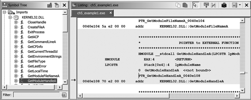
Figure 5-14: Import address table entry and associated location in Listing window
An important point to remember about the Imports category is that it displays only the symbols named in the binary’s import table. Symbols that a binary chooses to load on its own using a mechanism such as dlopen/dlsym or LoadLibrary/GetProcAddress will not be listed in the Symbol Tree window.
Exports
The Exports folder lists the entry points into the file. These include the program’s execution entry point, as specified in its header section, along with any functions and variables that the file exports for use by other files. Exported functions are commonly found in shared libraries such as Windows DLL files. Exported entries are listed by name, and the corresponding virtual address will be highlighted in the Listing window when the export is selected. For executable files, the Exports folder always contains at least one entry: the program’s execution entry point. Ghidra may name this symbol entry or _start, depending on the binary’s type.
Functions
The Functions folder contains a list of every function that Ghidra has identified in the binary. Hovering over a function name in the Symbol Tree window generates a pop-up with detailed information about the function, as shown in Figure 5-15. As part of the loading process, the loader utilizes various algorithms, including file structure analysis and byte sequence matching to infer the compiler that was used to create the file. During the analysis phase, the Function ID analyzer utilizes the compiler identification information to perform hash-based function body matching in order to identify the presence of library function bodies that may have been linked into the binary. When a hash match is made, Ghidra retrieves the matched function’s name from the hash database (contained in Ghidra .fidbf files) and adds the name as a function symbol. Hash matching is particularly useful on stripped binaries, as it provides a means of symbol recovery that is independent of the presence of a symbol table. This functionality is discussed in more depth in “Function IDs” on page 272.

Figure 5-15: Symbol Tree Functions folder pop-up
Labels
The Labels folder is the data equivalent of the Functions folder. Any data symbols contained in a binary’s symbol table will be listed in the Labels folder. In addition, anytime you add a new label name to a data address, that label will be added to the Labels folder.
Classes
The Classes folder contains an entry for each class identified by Ghidra during its analysis phase. Under each, Ghidra lists the identified data and methods that may assist you in understanding the behavior of the class. C++ classes and the structures that Ghidra uses to populate the classes folder are discussed in more detail in Chapter 8.
Namespaces
In the Namespaces folder, Ghidra may create new namespaces to provide organization and ensure that assigned names do not conflict in the binary. For example, a namespace may be created for each identified external library or for each switch statement that uses jump tables (allowing jump table labels to be reused in other switch statements without conflicting).
The Data Type Manager Window
The Data Type Manager window allows you to locate, organize, and apply data types to your file by using a system of data type archives. Archives represent Ghidra’s accumulated knowledge of predefined data types gleaned from header files included with most popular compilers. By processing header files, Ghidra understands the data types that are expected by common library functions and can annotate your disassembly and decompiler listings accordingly. Similarly, from these header files, Ghidra understands both the size and layout of complex data structures. All of this information is collected into archive files and applied anytime a binary is analyzed.
Referring back to Figure 5-4, you can see that the root of the BuiltInTypes tree, which contains primitive types like int that cannot be changed, renamed, or moved within a data type archive, is displayed in the Data Type Manager window (bottom left of the CodeBrowser window) even without a program loaded. In addition to the built-in types, Ghidra supports the creation of user-defined data types, including structures, unions, enums, and typedefs. It also supports arrays and pointers as derived data types.
Each file you open has an associated entry in the Data Type Manager window, as shown previously in Figure 5-5. The folder shares the name of the current file and entries within the folder are specific to the current file.
The Data Type Manager window displays nodes for each of the data type archives that are open. Archives can be opened automatically, such as when a program references an archive, or manually by the user. Data types and the Data Type Manager are covered in more detail in Chapters 8 and 13.
The Console Window
The Console window at the bottom of the CodeBrowser window serves as Ghidra’s output area for plugins and scripts, including those you develop yourself, and is the place to look for information on tasks Ghidra is performing as you work with a file. Developing scripts and plugins is introduced in Chapters 14 and 15.
The Decompiler Window
The Decompiler window allows you to simultaneously view and manipulate assembly and C representations of your binary through connected windows. The C representation that is generated by the Ghidra decompiler isn’t always perfect, but it can be very useful in helping you to understand a binary. Basic functionality provided by the decompiler includes recovery of expressions, variables, function parameters, and structure fields. The decompiler is also often capable of recovering a function’s block structure, which tends to get obscured in assembly language, which is not block structured and makes extensive use of goto (or equivalent) statements to appear block structured.
The Decompiler window displays a C representation of a function selected in the Listing window, as shown in Figure 5-16. Depending on your experience with assembly language, the decompiled code may be much easier to understand than the code in the Listing window. Even beginning programmers should be able to identify the infinite loop in the decompiled function. (The while loop condition is dependent on the value of param_3, which is not modified within the loop.)
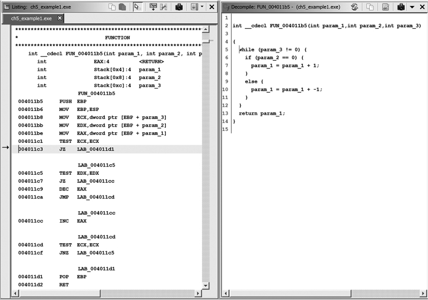
Figure 5-16: Listing and Decompiler windows
The Decompiler window icons are shown in Figure 5-17. You can use the Snapshot icon to open additional (disconnected) Decompiler windows if you want to compare the decompiled version of multiple functions or continue viewing a particular function while moving elsewhere in the Listing window. The Export icon allows you to save the decompiled function to a C file.
Within the Decompiler window, context menus are available through right-clicking that allow you to perform actions associated with a highlighted item. The options associated with one of the function parameters, param_1, are shown in Figure 5-18.

Figure 5-17: Decompiler window toolbar

Figure 5-18: Decompiler window options for function parameters
Decompilation is an extraordinarily complicated process, and decompiler theory remains an active research area. Unlike disassembly, whose accuracy can be verified against manufacturers’ reference manuals, there are no reference manuals that provide canonical translations of assembly language back to C (or C to assembly for that matter). In fact, while Ghidra’s decompiler always generates C source code, it may be the case that the binary the decompiler is analyzing was originally written in a language other than C, and many of the decompiler’s C-oriented assumptions may not hold at all.
As with most complex plugins, the decompiler has idiosyncrasies, and the quality of its output depends, to a large extent, on the quality of its input. Many of the issues and irregularities in the Decompiler window can be traced back to issues with the underlying disassembly, so if the decompiled code doesn’t make sense, you may need to spend time improving the quality of the disassembly. In most cases, this involves annotating the disassembly with more accurate data type information, which is discussed in Chapters 8 and 13. We continue to explore the decompiler’s capabilities in subsequent chapters and discuss it in depth in Chapter 19.
Other Ghidra Windows
In addition to the six default windows, you can open other windows to support your SRE process with alternate or specialized views into the file. The list of available windows is displayed from the Window menu, shown previously in Figure 5-4. The utility of these displays depends on both the characteristics of the binary you are analyzing and your skill with Ghidra. Several of these windows are sufficiently specialized to require more detailed coverage in later chapters, but we introduce some common ones here.
The Bytes Window
The Bytes window provides a raw look at the byte-level content of the file. By default, the Bytes window opens on the upper-right side of the CodeBrowser and provides a standard hex dump display of the program contents with 16 bytes per line. The window doubles as a hex editor and can be configured to display a variety of formats by using the Settings tool in the Bytes window toolbar. In many cases, it might be helpful to add the ASCII display to the Bytes window, as shown in Figure 5-19. The figure also shows the Byte Viewer Options dialog and toolbar icons for editing or snapshotting the byte view.
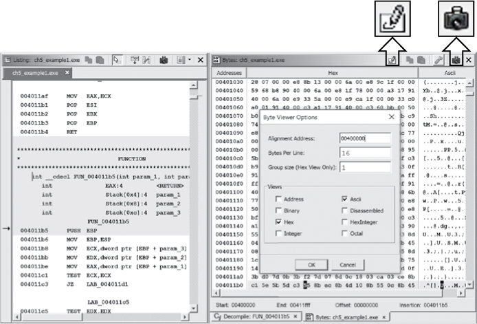
Figure 5-19: Synchronized hex and disassembly views with Toggle and Snapshot icons emphasized
As with the Listing window, several Bytes windows can be opened simultaneously using the Snapshot icon (see Figure 5-19) in the Bytes window toolbar. By default, the first Bytes window has a connection to the Listing window, so scrolling in one window and clicking an element causes the other window to scroll to the same location (same virtual address). Subsequent Bytes windows are disconnected, which allows you to scroll through them independently. When a window is disconnected, the window name appears within square brackets in the window title bar.
To turn the Bytes window into a hex (or ASCII) editor, simply toggle the pencil icon highlighted in Figure 5-19. The cursor will turn red to indicate that you can edit, though you will not be able to edit at addresses that contain an existing code item such as an instruction. When you are finished editing, toggle the icon again and you will be back in read-only mode. (Note that any changes will not be reflected in disconnected Bytes windows.)
If the Hex column displays question marks rather than hex values, Ghidra is telling you that it is not sure what values might occupy a given virtual address range. Such is the case when a program contains a bss section,4 which typically occupies no space within a file but is expanded by the loader to accommodate the program’s static storage requirements.
The Defined Data Window
The Defined Data window displays a string representation of data defined in the current program, view, or selection, along with the associated address, type, and size, as shown in Figure 5-20. As with most of the columnar windows, you can sort by any column in ascending or descending order by clicking the column header. Double-clicking any row in the Defined Data window causes the Listing window to jump to the address of the selected item.
When used with cross-references (discussed in Chapter 9), the Defined Data window provides the means to rapidly spot an interesting item and to track back to any location in the program that references that item with only a few clicks. For example, you might see the string "SOFTWAREMicrosoftWindowsCurrent VersionRun" listed and wonder why an application is referencing this particular key within the Windows registry, and then discover that the program is setting that registry key to automatically start itself when Windows boots.

Figure 5-20: Defined Data window with Filter icon emphasized
The Defined Data window has extensive filtering capabilities. In addition to the Filter bar at the bottom of the window, a Filter icon at the top right (emphasized in Figure 5-20) allows you to control additional data type filter options, as shown in Figure 5-21.

Figure 5-21: Defined data type filter options
Every time you close the Set Data Type Filter dialog by clicking OK, Ghidra will regenerate the Defined Data window contents in accordance with the new settings.
The Defined Strings Window
The Defined Strings window displays strings that have been defined in the binary. An example of this window is shown in Figure 5-22. In addition to the default columns displayed in the figure, you can add columns by right-clicking in the row of column titles. Perhaps one of the most interesting available columns is the Has Encoding Error flag, which can be indicative of an issue with the character set or misidentification of a string. In addition to this window, substantial string search functionality is available in Ghidra. This is discussed in Chapter 6.
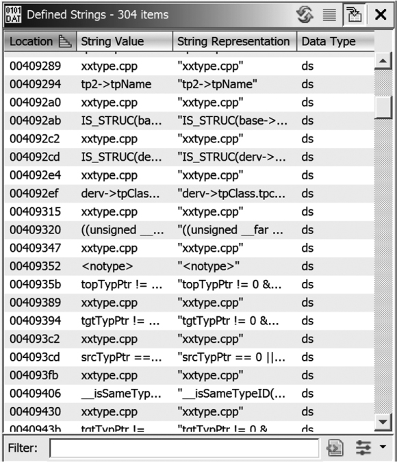
Figure 5-22: Defined Strings window
The Symbol Table and Symbol References Windows
The Symbol Table window provides a summary listing of all the global names within a binary. Eight columns are displayed by default, as shown in Figure 5-23. The window is highly configurable, with the capability to add and delete columns in the display as well as to sort in ascending or descending order on any column. The first two default columns are Name and Location. A name is nothing more than a symbolic description given to a symbol defined at a location.
The Symbol Table is connected to the Listing window but provides the capability to control its interaction with the Listing window. The emphasized icon on the right in Figure 5-23 is a toggle that determines whether a single click on a location in the Symbol Table window causes a related move in the Listing window. Regardless of the toggle selection, double-clicking any Symbol Table location entry will immediately jump the Listing view to display the selected entry. This provides a useful tool for rapidly navigating to known locations within a program listing.

Figure 5-23: Symbol Table window with Display Symbol References and Navigation Toggle icons emphasized
There is extensive filtering capability available in the Symbol Table window and several ways to access the filtering options. The cog icon in the toolbar opens the Symbol Table Filter dialog. The dialog (with the Use Advanced Filters box checked) is shown in Figure 5-24. In addition to this dialog, you can use the Filter options at the bottom of the window. Thorough discussions of the symbol table filtering options are available in Ghidra Help.
The emphasized icon on the left in Figure 5-23 is the Display Symbol References icon. Clicking this icon adds the Symbol References window to the Symbol Table window. By default, these two tables will appear side by side. To improve readability, you can drag the Symbol References window below the Symbol Table window, as shown in Figure 5-25. The connection between these two tables is unidirectional, with the Symbol References table being updated when a selection is made in the Symbol Table.
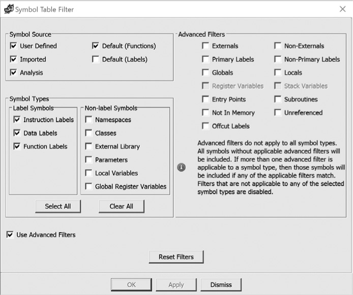
Figure 5-24: Symbol Table Filter dialog

Figure 5-25: Symbol Table with Symbol References
Like the Symbol Table window, the Symbol References window has the same column organization controls. In addition, the content of the Symbol References window is controlled by the three icons (S, I, and D) at the top right of the Symbol References toolbar. These options are mutually exclusive, meaning only one can be selected at a time:
S icon When this icon is selected, the Symbol References window will display all references to the symbol that you have selected in the Symbol Table. Figure 5-25 shows a Symbol References window with this option selected.
I icon When this icon is selected, the Symbol References window will display all instruction references from the function that you have selected in the Symbol Table. (This list will be empty if you did not select a function entry point.)
D icon When this icon is selected, the Symbol References window will display all data references from the function that you have selected in the Symbol Table. This list will be empty if you did not select a function entry point or if the function makes no references to any data symbols.
The Memory Map Window
The Memory Map window displays a summary listing of the memory blocks present in the program, as shown in Figure 5-26. Note that what Ghidra terms memory blocks are frequently called sections when discussing the structure of binary files. Information presented in the window includes the memory block (section) name, start and end addresses, length, permission flags, block type, initialized flag, as well as a space for source filename and user comments. The start and end addresses represent the virtual address range to which the program sections will be mapped at runtime.
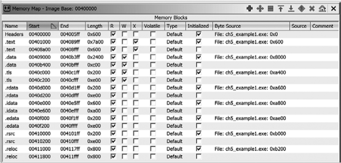
Figure 5-26: Memory Map window
Double-clicking any start or end address in the window jumps the Listing window (and all other connected windows) to the specified address. The Memory Map window toolbar provides options to add/delete blocks, move blocks, split/merge blocks, edit addresses, and set a new image base. These features are particularly useful when reverse engineering files with nonstandard formats, as the binary’s segment structure may not have been detected by the Ghidra loader.
Command line counterparts to the Memory Map window include objdump (-h), readelf (-S), and dumpbin (/HEADERS).
The Function Call Graph Window
In any program, a function can both call and be called by other functions. The Function Call Graph window shows the immediate neighbors of a given function. For our purposes, we will call Y a neighbor of X if Y directly calls X or if X directly calls Y. When you open the Function Call Graph window, Ghidra determines the neighbors of the function in which the cursor is positioned and generates the associated display. This display shows a function in the context it is used in the program file, but it is just a part of the big picture.
Figure 5-27 shows a function named FUN_0040198c that is called from FUN_00401edc and, in turn, makes calls to six other functions. Double-clicking any function in the window immediately jumps the Listing window and other connected windows to the selected function. Ghidra cross-references (XREFs) are the mechanisms that underlie the generation of the Function Call Graph window. XREFs are covered in more detail in Chapter 9.
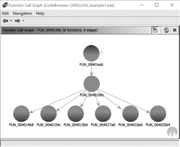
Figure 5-27: Function Call Graph window
WHO’S CALLING?
While the Function Call Graph window is helpful, sometimes you need the big picture, or at least a bigger picture. The Function Call Trees window (Window ▸ Function Call Trees) allows you to see all calls to and from a selected function. The Function Call Trees window (as shown in Figure 5-28) has two sections: one for incoming calls and one for outgoing calls. Both incoming and outgoing calls can be expanded and collapsed, as desired.
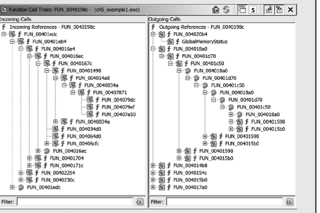
Figure 5-28: The Function Call Trees view
If you open the Function Call Tree window with the entry function selected, you can view a hierarchical representation of the program’s function calls.
Summary
At first glance, the number of displays that Ghidra offers can seem overwhelming. You may find it easiest to stick with the default displays until you are comfortable enough to begin exploring the additional display offerings. In any case, you should certainly not feel obligated to use everything that Ghidra throws at you. Not every window will be useful in every reverse engineering scenario.
One of the best ways to familiarize yourself with Ghidra’s displays is simply to browse around the various tabbed subwindows that Ghidra populates with data about your binary and also open a few of the other available windows. The efficiency and effectiveness of your reverse engineering sessions will improve as your comfort level with Ghidra increases.
Ghidra is a very complex tool. In addition to the windows covered in this chapter, you may encounter additional dialogs as you endeavor to master Ghidra. We introduce key dialogs as they become relevant throughout the remainder of the book.
At this point, you should be starting to feel more comfortable with the Ghidra interface and the CodeBrowser desktop. In the next chapter, we begin to focus on the many ways that you can manipulate a disassembly to enhance your understanding of its behavior and to generally make your life easier with Ghidra.