20
COMPILER VARIATIONS

At this point, if we have done our job properly, you now possess the essential skills to use Ghidra effectively and, more importantly, to bend it to your will. The next step is to learn to adapt to the challenges that binaries (as opposed to Ghidra) will throw at you. Depending on your motives for staring at assembly language, either you may be very familiar with what you are looking at or you may never know what you are going to be faced with. If you spend all of your time examining code that was compiled using gcc on a Linux platform, you’ll become quite familiar with the style of code that it generates, but you may be baffled by a debug version of a program compiled using the Microsoft C/C++ compiler. If you are a malware analyst, you may see code created using gcc, clang, Microsoft's C++ compiler, Delphi, and others, all in the same afternoon.

Like you, Ghidra is more familiar with the output of some compilers than other compilers, and familiarity with code generated by one compiler in no way guarantees that you will recognize high-level constructs compiled using an entirely different compiler (or even different versions of the same compiler family). Rather than relying entirely on Ghidra’s analysis capabilities to recognize commonly used code and data constructs, you should always be prepared to utilize your own skills: your familiarity with a given assembly language, your knowledge of compilers, and your research skills to properly interpret a disassembly.

In this chapter, we cover some of the ways that compiler differences manifest themselves in disassembly listings. We primarily use compiled C code for our examples, as the variability of C compilers and target platforms provides foundational concepts that can be extended to other compiled languages.

High-Level Constructs

In some cases, the differences between compilers may just be cosmetic, but in other cases, they are much more significant. In this section, we look at high-level language constructs and demonstrate how different compilers and compiler options may significantly impact the resulting disassembly listing. We begin with switch statements and the two mechanisms most commonly employed to resolve switch case selection. Following that, we look at the way that compiler options affect code generation for common expressions before moving on to discuss how different compilers implement C++-specific constructs and handle program startup.

switch Statements

The C switch statement is a frequent target for compiler optimizations. The goal of these optimizations is to match the switch variable to a valid case label in the most efficient manner possible, but the distribution of the switch statement’s case labels constrains the type of search that can be used.

Since the efficiency of a search is measured by the number of comparisons required to find the correct case, we can trace the logic a compiler might use to determine the best way to represent a switch table. A constant time algorithm, such as a table lookup, is the most efficient.¹ At the other end of the continuum is linear search, which, in the worst case, requires comparing the switch variable against every case label before finding a match or resolving to the default and thus is the least efficient.² The efficiency of a binary search is much better, on average, than linear search but introduces additional constraints, as it requires a sorted list.³

In order to select the most efficient implementation for a particular switch statement, it helps to understand how the case label distribution affects the compiler’s decision-making process. When case labels are closely clustered, as in the source code in Listing 20-1, compilers generally resolve the switch variable by performing a table lookup to match the switch variable to the address of its associated case—specifically by using a jump table.

switch (a) {
/** NOTE: case bodies omitted for brevity **/
    case 1:  /*...*/ break;
    case 2:  /*...*/ break;
    case 3:  /*...*/ break;
    case 4:  /*...*/ break;
    case 5:  /*...*/ break;
    case 6:  /*...*/ break;
    case 7:  /*...*/ break;
    case 8:  /*...*/ break;
    case 9:  /*...*/ break;
    case 10: /*...*/ break;
    case 11: /*...*/ break;
    case 12: /*...*/ break;
}

Listing 20-1: A switch statement with consecutive case labels

A jump table is an array of pointers, with each pointer in the array referencing a possible jump target. At runtime, a dynamic index into the table chooses one of the many potential jumps each time the jump table is referenced. Jump tables work well when switch case labels are closely spaced (dense), with most of the cases falling into a consecutive number sequence. Compilers take this into account when deciding whether to utilize a jump table. For any switch statement, we can compute the minimum number of entries an associated jump table will contain as follows:

num_entries = max_case_value – min_case_value + 1

The density, or utilization rate, of the jump tables can then be computed as follows:

density = num_cases / num_entries

A completely contiguous list with every value represented would have a density value of 100 percent (1.0). Finally, the total amount of space required to store the jump table is as follows:

table_size = num_entries * sizeof(void*)

A switch statement with 100 percent density will be implemented using a jump table. A set of cases with a density of 30 percent might not be implemented using a jump table, since jump table entries would still need to be allocated for the absent cases, which would be 70 percent of the jump table. If num_entries is 30, the jump table would contain entries for 21 unreferenced case labels. On a 64-bit system, this is 168 of the 240 bytes allocated to the table, which is not a lot of overhead, but if num_entries jumps to 300, then the overhead becomes 1680 bytes, which may not be worth the trade-off for 90 possible cases. A compiler that is optimizing for speed may favor jump table implementations, while a compiler that is optimizing for size may choose an alternative implementation with lower memory overhead: binary search.

Binary search is efficient when the case labels are widely spread (low density), as seen in Listing 20-2 (density 0.0008).⁴ Because binary search works only on sorted lists, the compiler must ensure that the case labels are ordered before it begins the search with the median value. This may result in the reordering of case blocks when viewed in a disassembly, as compared to the order they appear in the corresponding source.⁵

switch (a) {
/** NOTE: case bodies omitted for brevity **/
    case 1:     /*...*/ break;
    case 211:   /*...*/ break;
    case 295:   /*...*/ break;
    case 462:   /*...*/ break;
    case 528:   /*...*/ break;
    case 719:   /*...*/ break;
    case 995:   /*...*/ break;
    case 1024:  /*...*/ break;
    case 8000:  /*...*/ break;
    case 13531: /*...*/ break;
    case 13532: /*...*/ break;
    case 15027: /*...*/ break;
}

Listing 20-2: Sample switch statement with nonconsecutive case labels

Listing 20-3 shows an outline for a non-iterative binary search through a fixed number of constant values. This is the rough framework that the compiler uses to implement the switch from Listing 20-2.

if (value < median) {
    // value is in [0-50) percentile
    if (value < lower_half_median) {
        // value is in [0-25) percentile
        // ... continue successive halving until value is resolved
    } else {
        // value is in [25-50) percentile
        // ... continue successive halving until value is resolved
   }
} else {
    // value is in [50-100) percentile
    if (value < upper_half_median) {
        // value is in [50-75) percentile
        // ... continue successive halving until value is resolved
    } else {
        // value is in [75-100) percentile
        // ... continue successive halving until value is resolved
    }
}

Listing 20-3: Non-iterative binary search through a fixed number of constant values

Compilers are also capable of performing more fine-grained optimizations across a range of case labels. For example, when confronted with the case labels

label_set = [1, 2, 3, 4, 5, 6, 7, 8, 50, 80, 200, 500, 1000, 5000, 10000]

a less aggressive compiler might see a density of 0.0015 here and generate a binary search through all 15 cases. A more aggressive compiler might emit a jump table to resolve cases 1 to 8, and a binary search for the remaining cases, achieving optimal performance for over half of the cases.

Before we look at the disassembled versions of Listings 20-1 and 20-2, let’s look at the Ghidra Function Graph windows corresponding to the listings, shown side by side in Figure 20-1.

Figure 20-1: Ghidra Function Graph switch statement examples

On the left, the graph for Listing 20-1 shows a nice vertical stack of cases. Each stacked code block resides at the same nesting depth, as is true for cases in a switch statement. The stack suggests that we can use an index to quickly select one block from the many (think array access). This is precisely how jump table resolution works, and the left-hand graph provides us with a visual hint that this is the case, even before we have looked at a single line of the disassembly.

The right-hand graph is Ghidra’s result based solely on its understanding of the disassembly of Listing 20-2. The lack of a jump table makes it much more challenging to identify this as a switch statement. What you are seeing is a visual representation of the switch statement using Ghidra’s Nested Code Layout. This is the default layout for function graphs in Ghidra and is intended to represent the flow structures in a program. The horizontal branching in this graph suggests conditional execution (if/else) branching to mutually exclusive alternatives. The vertical symmetry suggests that the alternative execution paths have been very carefully balanced to place equal numbers of blocks in each vertical half of the graph. Finally, the distance that the graph traverses horizontally is an indicator of the depth reached by the search, which in turn is dictated by the total number of case labels present in the switch. For a binary search, this depth will always be on the order of log₂(num_cases). The similarity between the indentation of the graphical representation and the algorithm outlined in Listing 20-3 is easily observable.

Turning our attention to the Decompiler window, Figure 20-2 shows the partial decompilation of the functions displayed in Figure 20-1. On the left is the decompiled version of Listing 20-1. As with the graph, the presence of a jump table in the binary helps Ghidra identify the code as a switch statement.

On the right is the decompiled version of Listing 20-2. The decompiler has presented the switch statement as a nested if/else structure consistent with a binary search, and similar in structure to Listing 20-3. You can see that first comparison is against 719, the median value in the list, and that subsequent comparisons continue to divide the search space in half. Referring to Figure 20-1 (as well as Listing 20-3), we can again observe that the graphical representations of each function closely correspond to the indentation patterns observed in the Decompiler window.

Now that you have an idea of what is happening from a high level, let’s look inside the binaries and investigate what is happening at a low level. Since our objective in this chapter is to observe differences between compilers, we present this example as a series of comparisons between two compilers, gcc and Microsoft C/C++.⁶

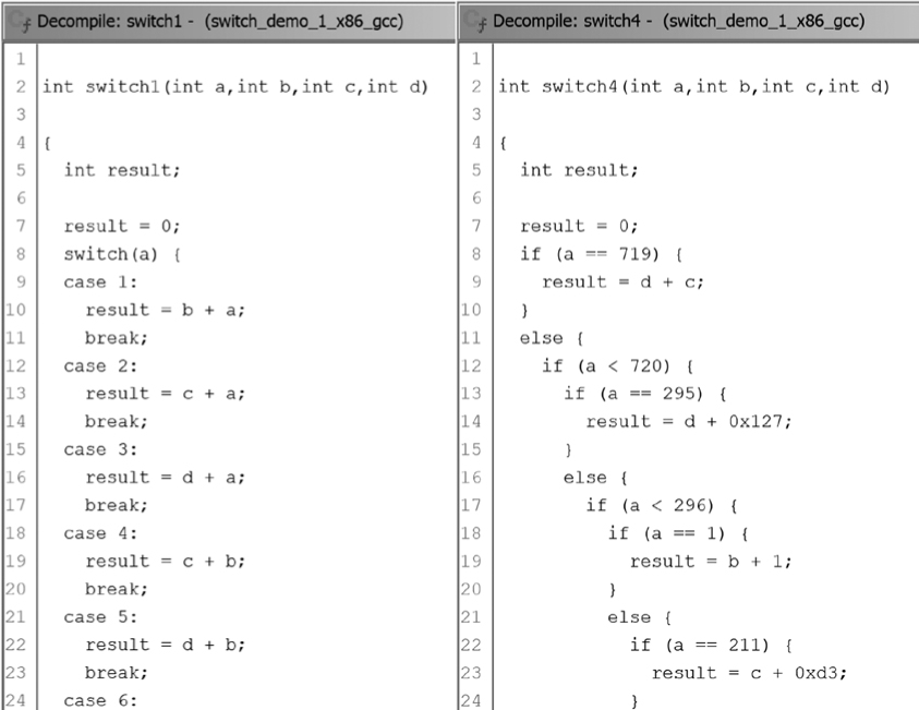
Figure 20-2: Ghidra decompiled switch statement examples

Example: Comparing gcc with Microsoft C/C++ Compiler

In this example, we compare two 32-bit x86 binaries generated for Listing 20-1 by two distinct compilers. We will attempt to identify components of a switch statement in each binary, locate the associated jump table in each binary, and point out significant differences between the two binaries. Let’s start by looking at the switch-related components for Listing 20-1 in the binary built with gcc:

0001075a  CMP➊  dword ptr [EBP + value],12
0001075e  JA     switchD_00010771::caseD_0➋
00010764  MOV    EAX,dword ptr [EBP + a]
00010767  SHL    EAX,0x2
0001076a  ADD    EAX,switchD_00010771::switchdataD_00010ee0       = 00010805
0001076f  MOV    EAX,dword ptr [EAX]=>->switchD_00010771::caseD_0 = 00010805
        switchD_00010771::switchD
00010771  JMP    EAX
        switchD_00010771::caseD_1➌             XREF[2]:      00010771(j), 00010ee4(*)
00010773  MOV    EDX,dword ptr [EBP + a]
00010776  MOV    EAX,dword ptr [EBP + b]
00010779  ADD    EAX,EDX
0001077b  MOV    dword ptr [EBP + result],EAX
0001077e  JMP    switchD_00010771::caseD_0
;--content omitted for remaining cases--
       switchD_00010771::switchdataD_00010ee0➋  XREF[2]: switch_version_1:0001076a(*),
                                                          switch_version_1:0001076f(R)
00010ee0  addr    switchD_00010771::caseD_0➎
00010ee4  addr    switchD_00010771::caseD_1
00010ee8  addr    switchD_00010771::caseD_2
00010eec  addr    switchD_00010771::caseD_3
00010ef0  addr    switchD_00010771::caseD_4
00010ef4  addr    switchD_00010771::caseD_5
00010ef8  addr    switchD_00010771::caseD_6
00010efc  addr    switchD_00010771::caseD_7
00010f00  addr    switchD_00010771::caseD_8
00010f04  addr    switchD_00010771::caseD_9
00010f08  addr    switchD_00010771::caseD_a
00010f0c  addr    switchD_00010771::caseD_b
00010f10  addr    switchD_00010771::caseD_c

Ghidra recognizes the switch bounds test ➊, the jump table ➍, and individual case blocks by value, such as the one at switchD_00010771::caseD_1 ➌. The compiler generated a jump table with 13 entries, although Listing 20-1 contained only 12 cases. The additional case, case 0 (the first entry ➎ in the jump table), shares a target address with every value outside the range 1 to 12. In other words, case 0 is part of the default case. While it may seem that negative numbers are being excluded from the default, the CMP, JA sequence works as a comparison on unsigned values; thus, -1 (0xFFFFFFFF) would be seen as 4294967295, which is much larger than 12 and therefore excluded from the valid range for indexing the jump table. The JA instruction directs all such cases to the default location: switchD_00010771::caseD_0 ➋.

Now that we understand the basic components of the code generated by the gcc compiler, let’s shift our focus to the same components in code generated by the Microsoft C/C++ compiler in debug mode:

00411e88  MOV    ECX,dword ptr [EBP + local_d4]
00411e8e  SUB➊  ECX,0x1
00411e91  MOV    dword ptr [EBP + local_d4],ECX
00411e97  CMP➋  dword ptr [EBP + local_d4],11
00411e9e  JA     switchD_00411eaa::caseD_c
00411ea4  MOV    EDX,dword ptr [EBP + local_d4]
        switchD_00411eaa::switchD
00411eaa  JMP    dword ptr [EDX*0x4 + ->switchD_00411eaa::caseD      = 00411eb1
        switchD_00411eaa::caseD_1                XREF[2]: 00411eaa(j), 00411f4c(*)
00411eb1  MOV    EAX,dword ptr [EBP + param_1]
00411eb4  ADD    EAX,dword ptr [EBP + param_2]
00411eb7  MOV    dword ptr [EBP + local_c],EAX
00411eba  JMP    switchD_00411eaa::caseD_c
;--content omitted for remaining cases--
        switchD_00411eaa::switchdataD_00411f4c   XREF[1]: switch_version_1:00411eaa(R)
00411f4c  addr   switchD_00411eaa::caseD_1➌
00411f50  addr   switchD_00411eaa::caseD_2
00411f54  addr   switchD_00411eaa::caseD_3
00411f58  addr   switchD_00411eaa::caseD_4
00411f5c  addr   switchD_00411eaa::caseD_5
00411f60  addr   switchD_00411eaa::caseD_6
00411f64  addr   switchD_00411eaa::caseD_7
00411f68  addr   switchD_00411eaa::caseD_8
00411f6c  addr   switchD_00411eaa::caseD_9
00411f70  addr   switchD_00411eaa::caseD_a
00411f74  addr   switchD_00411eaa::caseD_b
00411f78  addr   switchD_00411eaa::caseD_c

Here, the switch variable (local_d4 in this case) is decremented ➊ to shift the range of valid values from 0 to 11 ➋, eliminating the need for a dummy table entry for the value 0. As a result, the first entry (or 0 index entry) in the jump table ➌ actually refers to the code for switch case 1.

Another, perhaps more subtle difference between the two listings is the location of the jump table within the file. The gcc compiler places switch jump tables in the read-only data (.rodata) section of the binary, providing a logical separation between the code associated with the switch statement and the data required to implement the jump table. The Microsoft C/C++ compiler, on the other hand, inserts jump tables into the .text section, immediately following the function containing the associated switch statement. Positioning the jump table in this manner has little effect on the behavior of the program. In this example, Ghidra is able to recognize the switch statements for both compilers and uses the term switch within the associated labels.

One of the key points here is that there is no single correct way to compile source to assembly. As a result, you cannot assume that something is not a switch statement simply because Ghidra fails to label it as such. Understanding the switch statement characteristics that factor into the compiler implementation can help you make a more accurate inference about the original source code.

Compiler Build Options

A compiler converts high-level code that solves a particular problem into low-level code that solves the same problem. Multiple compilers may solve the same problem in rather different ways. Further, a single compiler may solve a problem very differently based on the associated compiler options. In this section, we look at the assembly language code that results from using different compilers and different command line options. (Some differences will have a clear explanation; others will not.)

Microsoft’s Visual Studio can build either debug or release versions of program binaries.⁷ To see how the two versions are different, compare the build options specified for each. Release versions are generally optimized, while debug versions are not, and debug versions are linked with additional symbol information and debugging versions of the runtime library, while release versions are not.⁸ Debugging-related symbols allow debuggers to map assembly language statements back to their source code counterparts and to determine the names of local variables (such information is otherwise lost during the compilation process). The debugging versions of Microsoft’s runtime libraries have also been compiled with debugging symbols included, optimizations disabled, and additional safety checks enabled to verify that some function parameters are valid.

When disassembled using Ghidra, debug builds of Visual Studio projects look significantly different from release builds. This is a result of compiler and linker options specified only in debug builds, such as basic runtime checks (/RTCx), which introduce extra code into the resulting binary.⁹ Let’s jump right in and look at some of these differences in disassemblies.

Example 1: Modulo Operator

We begin our examples with a simple mathematical operation, modulo. The following listing contains the source code for a program whose only goal is to accept an integer value from the user and demonstrate integer division and the modulo operator:

int main(int argc, char **argv) {
    int x;
    printf("Enter an integer: ");
    scanf("%d", &x);
    printf("%d %% 10 = %d ", x, x % 10);
}

Let’s investigate how the disassembly varies across compilers for the modulo operator in this example.

Modulo with Microsoft C/C++ Win x64 Debug

The following listing shows the code that Visual Studio generates when configured to build a debug version of the binary:

1400119c6 MOV    EAX,dword ptr [RBP + local_f4]
1400119c9 CDQ
1400119ca MOV    ECX,0xa
1400119cf IDIV➊ ECX
1400119d1 MOV    EAX,EDX
1400119d3 MOV➋  R8D,EAX
1400119d6 MOV    EDX,dword ptr [RBP + local_f4]
1400119d9 LEA    RCX,[s_%d_%%_10_=_%d_140019d60]
1400119e0 CALL   printf

A straightforward x86 IDIV instruction ➊ leaves the quotient in EAX and the remainder of the division in EDX. The result is then moved to lower 32 bits of R8 (R8D) ➋, which is the third argument in the call to printf.

Modulo with Microsoft C/C++ Win x64 Release

Release builds optimize software for speed and size in order to enhance performance and minimize storage requirements. When optimizing for speed, compiler writers may resort to non-obvious implementations of common operations. The following listing shows us how Visual Studio generates the same modulo operation in a release binary:

140001136 MOV    ECX,dword ptr [RSP + local_18]
14000113a MOV    EAX,0x66666667
14000113f IMUL➊ ECX
140001141 MOV    R8D,ECX
140001144 SAR    EDX,0x2
140001147 MOV    EAX,EDX
140001149 SHR    EAX,0x1f
14000114c ADD    EDX,EAX
14000114e LEA    EAX,[RDX + RDX*0x4]
140001151 MOV    EDX,ECX
140001153 ADD    EAX,EAX
140001155 LEA    RCX,[s_%d_%%_10_=_%d_140002238]
14000115c SUB➋  R8D,EAX
14000115f CALL➌ printf

In this case, multiplication ➊ is used rather than division, and after a long sequence of arithmetic operations, what must be the result of the modulo operation ends up in R8D ➋ (again the third argument in the call to printf ➌). Intuitive, right? An explanation of this code follows our next example.

Modulo with gcc for Linux x64

We’ve seen how differently one compiler can behave simply by changing the compile-time options used to generate a binary. We might expect that a completely unrelated compiler would generate entirely different code yet again. The following disassembly shows us the gcc version of the same modulus operation, and it turns out to look somewhat familiar:

00100708  MOV    ECX,dword ptr [RBP + x]
0010070b  MOV    EDX,0x66666667
00100710  MOV    EAX,ECX
00100712  IMUL➊ EDX
00100714  SAR    EDX,0x2
00100717  MOV    EAX,ECX
00100719  SAR    EAX,0x1f
0010071c  SUB    EDX,EAX
0010071e  MOV    EAX,EDX
00100720  SHL    EAX,0x2
00100723  ADD    EAX,EDX
00100725  ADD    EAX,EAX
00100727  SUB    ECX,EAX
00100729  MOV➋  EDX,ECX

The code is very similar to the assembly produced by the Visual Studio release version. We again see multiplication ➊ rather than division followed by a sequence of arithmetic operations that eventually leaves the result in EDX ➋ (where it is eventually used as the third argument to printf).

The code is using a multiplicative inverse to perform division by multiplying because hardware multiplication is faster than hardware division. You may also see multiplication implemented using a series of additions and arithmetic shifts, as each of these operations is significantly faster in hardware than multiplication.

Your ability to recognize this code as modulo 10 depends on your experience, patience, and creativity. If you’ve seen similar code sequences in the past, you are probably more apt to recognize what’s taking place here. Lacking that experience, you might instead work through the code manually with sample values, hoping to recognize a pattern in the results. You might even take the time to extract the assembly language, wrap it in a C test harness, and do some high-speed data generation to assist you. Ghidra’s decompiler can be another useful resource for reducing complex or unusual code sequences to their more recognizable C equivalents.

As a last resort, or first resort (don’t be ashamed), you might turn to the internet for answers. But what should you be searching for? Usually, unique, specific searches yield the most relevant results, and the most unique feature in the sequence of code is the integer constant 0x66666667. When we searched for this constant, the top three results were all helpful, but one in particular was worth bookmarking: http://flaviojslab.blogspot.com/2008/02/integer-division.html. Unique constants are also used rather frequently in cryptographic algorithms, and a quick internet search may be all it takes to identify exactly what crypto routine you are staring at.

Example 2: The Ternary Operator

The ternary operator evaluates an expression and then yields one of two possible results, depending on the boolean value of that expression. Conceptually, the ternary operator can be thought of as an if/else statement (and can even be replaced with an if/else statement). The following intentionally unoptimized source code demonstrates the use of this operator:

int main() {
    volatile int x = 3;
    volatile int y = x * 13;
  ➊ volatile int z = y == 30 ? 0 : -1;
}

As for the behavior of the unoptimized code, the assignment into variable z ➊ could be replaced with the following if/else statement without changing the semantics of the program:

    if (y == 30) {
        z = 0;
    } else {
        z = -1;
    }

Let’s see how the ternary operator code is handled by different compilers and different compiler options.

Ternary Operator with gcc on Linux x64

gcc, with no options, generated the following assembly for the initialization of z:

00100616  MOV    EAX,dword ptr [RBP + y]
00100619  CMP➊  EAX,0x1e
0010061c  JNZ    LAB_00100625
0010061e  MOV    EAX,0x0
00100623  JMP    LAB_0010062a
        LAB_00100625
00100625  MOV    EAX,0xffffffff
        LAB_0010062a
0010062a  MOV➋  dword ptr [RBP + z],EAX

This code uses the if/else implementation. Local variable y is compared to 30 ➊ to decide whether to set EAX to 0 or 0xffffffff in opposing branches of the if/else before assigning the result into z ➋.

Ternary Operator with Microsoft C/C++ Win x64 Release

Visual Studio yields a very different implementation of the statement containing the ternary operator. Here, the compiler recognizes that a single instruction can be used to conditionally generate either 0 or -1 (and no other possible value) and uses this instruction in lieu of the if/else construct we saw earlier:

140001013 MOV    EAX,dword ptr [RSP + local_res8]
140001017 SUB➊  EAX,0x1e
14000101a NEG➋  EAX
14000101c SBB➌  EAX,EAX
14000101e MOV    dword ptr [RSP + local_res8],EAX

The SBB instruction ➌ (subtract with borrow) subtracts the second operand from the first operand and then subtracts the carry flag, CF (which can be only 0 or 1). The equivalent arithmetic expression to SBB EAX,EAX is EAX – EAX – CF, which reduces to 0 – CF. This, in turn, can result only in 0 (when CF == 0) or -1 (when CF == 1). For this trick to work, the compiler must set the carry properly prior to executing the SBB instruction. This is accomplished by comparing EAX to the constant 0x1e (30) ➊ using a subtraction that leaves EAX equal to 0 only when EAX was initially 0x1e. The NEG instruction ➋ then sets the carry flag for the SBB instruction that follows.¹⁰

Ternary Operator with gcc on Linux x64 (Optimized)

When we ask gcc to try a little harder by optimizing its code (-O2), the result is not unlike the Visual Studio code in the previous example:

00100506  MOV    EAX,dword ptr [RSP + y]
0010050a  CMP    EAX,0x1e
0010050d  SETNZ➊AL
00100510  MOVZX  EAX,AL
00100513  NEG➋  EAX
00100515  MOV➌  dword ptr [RSP + z],EAX

In this case, gcc uses SETNZ ➊ to conditionally set the AL register to either 0 or 1 based on the state of the zero flag resulting from the preceding comparison. The result is then negated ➋ to become either 0 or -1 before assignment into variable z ➌.

Example 3: Function Inlining

When a programmer marks a function inline, they are suggesting to the compiler that any calls to the function should be replaced with a copy of the entire function body. The intent is to speed up the function call by eliminating parameter and stack frame setup and teardown. The trade-off is that many copies of an inlined function make the binary larger. Inlined functions can be very difficult to recognize in binaries because the distinctive call instruction is eliminated.

Even when the inline keyword has not been used, compilers may elect to inline a function on their own initiative. In our third example, we are making a call to the following function:

int maybe_inline() {
    return 0x12abcdef;
}
int main() {
    int v = maybe_inline();
    printf("after maybe_inline: v = %08x ", v);return 0;
}

Function Call with gcc on Linux x86

After building a Linux x86 binary using gcc with no optimizations, we disassemble it to see the following listing:

00010775  PUSH   EBP
00010776  MOV    EBP,ESP
00010778  PUSH   ECX
00010779  SUB    ESP,0x14
0001077c  CALL➊ maybe_inline
00010781  MOV    dword ptr [EBP + local_14],EAX
00010784  SUB    ESP,0x8
00010787  PUSH   dword ptr [EBP + local_14]
0001078a  PUSH   s_after_maybe_inline:_v_=_%08x_000108e2
0001078f  CALL   printf

We can clearly see the call ➊ to the maybe_inline function in this disassembly, even though it is just a single line of code returning a constant value.

Optimized Function Call with gcc on Linux x86

Next, we look at an optimized (-O2) version of the same source code:

0001058a  PUSH   EBP
0001058b  MOV    EBP,ESP
0001058d  PUSH   ECX
0001058e  SUB    ESP,0x8
00010591  PUSH➊ 0x12abcdef
00010596  PUSH   s_after_maybe_inline:_v_=_%08x_000108c2
0001059b  PUSH   0x1
0001059d  CALL   __printf_chk

Contrasting this code with the unoptimized code, we see that the call to maybe_inline has been eliminated, and the constant value ➊ returned by maybe_inline is pushed directly onto the stack to be used as an argument for the call to printf. This optimized version of the function call is identical to what you would see if the function had been designated inline.

Having examined some of the ways that optimizations can influence the code generated by compilers, let’s turn our attention to the different ways that compiler designers choose to implement language-specific features when language designers leave implementation details to the compiler writers.

Compiler-Specific C++ Implementation

Programming languages are designed by programmers for programmers. Once the dust of the design process has settled, it’s up to compiler writers to build the tools that faithfully translate programs written in the new high-level language into semantically equivalent machine language programs. When a language permits a programmer to do A, B, and C, it’s up to the compiler writers to find a way to make these things possible.

C++ gives us three excellent examples of behaviors required by the language, but whose implementation details were left to the compiler writer to sort out:

• Within a nonstatic member function of a class, programmers may refer to a variable named this, which is never explicitly declared anywhere. (See Chapters 6 and 8 for compilers’ treatment of this.)

• Function overloading is allowed. Programmers are free to reuse function names as often as they like, subject to restrictions on their parameter lists.

• Type introspection is supported through the use of the dynamic_cast and typeid operators.

Function Overloading

Function overloading in C++ allows programmers to name functions identically, with the caveat that any two functions that share a name must have different parameter sequences. Name mangling, introduced in Chapter 8, is the under-the-hood mechanism that allows overloading to work by ensuring that no two symbols share the same name by the time the linker is asked to do its job.

Often, one of the earliest signs that you are working with a C++ binary is the presence of mangled names. The two most popular name mangling schemes are Microsoft’s and the Intel Itanium ABI.¹¹ The Intel standard has been widely adopted by other Unix compilers such as g++ and clang. The following shows a C++ function name and the mangled version of that name under both the Microsoft and Intel schemes:

Function void SubClass::vfunc1()

Microsoft scheme ?vfunc1@SubClass@@UAEXXZ

Intel scheme _ZN8SubClass6vfunc1Ev

Most languages that permit overloading, including Objective-C, Swift, and Rust, incorporate some form of name mangling at the implementation level. A passing familiarity with name-mangling styles can provide you with clues about a program’s original source language as well as the compiler used to build the program.

RTTI Implementations

In Chapter 8, we discussed C++ Runtime Type Identification (RTTI) and the lack of a standard for implementing RTTI by a compiler. In fact, runtime type identification is not mentioned anywhere in the C++ standard, so it should be no surprise that implementations differ. To support the dynamic_cast operator, RTTI data structures record not only a class’s name, but its entire inheritance hierarchy, including any multiple inheritance relationships. Locating RTTI data structures can be extremely useful in recovering the object model of a program. Automatic recognition of RTTI-related constructs within a binary is another area in which Ghidra’s capabilities vary across compilers.

Microsoft C++ programs contain no embedded symbol information, but Microsoft’s RTTI data structures are well understood, and Ghidra will locate them when present. Any RTTI-related information Ghidra does locate will be summarized in the Symbol Tree’s Classes folder, which will contain an entry for each class that Ghidra locates using its RTTI analyzer.

Programs built with g++ include symbol table information unless they have been stripped. For unstripped g++ binaries, Ghidra relies exclusively on the mangled names it finds in the binary, and it uses those names to identify RTTI-related data structures and the classes they are associated with. As with Microsoft binaries, any RTTI-related information will be included in the Symbol Tree’s Classes folder.

One strategy for understanding how a specific compiler embeds type information for C++ classes is to write a simple program that uses classes containing virtual functions. After compiling the program, you can load the resulting executable into Ghidra and search for instances of strings that contain the names of classes used in the program. Regardless of the compiler used to build a binary, one thing that RTTI data structures have in common is that they all reference, in some manner, a string containing the mangled name of the class that they represent. Using extracted strings and data cross-references, it should be possible to locate candidate RTTI-related data structures within the binary. The last step is to link a candidate RTTI structure back to the associated class’s vftable, which is best accomplished by following data cross-references backward from the candidate RTTI structure until a table of function pointers (the vftable) is reached. Let’s walk through an example that uses this method.

Example: Locating RTTI Information in a Linux x86-64 g++ Binary

To demonstrate these concepts, we created a small program with a BaseClass, a SubClass, a SubSubClass, and a collection of virtual functions unique to each. The following listing shows part of the main program we used to reference our classes and functions:

    BaseClass *bc_ptr_2;
    srand(time(0));
    if (rand() % 2) {
        bc_ptr_2 = dynamic_cast<SubClass*>(new SubClass());
    }
    else {
        bc_ptr_2 = dynamic_cast<SubClass*>(new SubSubClass());
    }

We compiled the program using g++ to build a 64-bit Linux binary with symbols. After we analyze the program, the Symbol Tree provides the information shown in Figure 20-3.

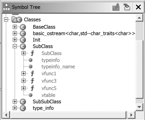
Figure 20-3: Symbol Tree classes for an unstripped binary

The Classes folder contains entries for all three of our classes. The expanded SubClass entry reveals additional information that Ghidra has uncovered about it. The stripped version of the same binary contains a lot less information, as shown in Figure 20-4.

Figure 20-4: Symbol Tree classes for a stripped binary

In this case, we might, incorrectly, assume that the binary contains no C++ classes of interest, although it is likely a C++ binary based on the reference to a core C++ class (basic_ostream). Since stripping removes only symbol information, we may still be able to find RTTI information by searching for class names in the program’s strings and walking our way back to any RTTI data structure. A string search yields the results shown in Figure 20-5.

Figure 20-5: String Search results revealing class names

If we click the "8SubClass" string, we are taken to this portion of the Listing window:

        s_8SubClass_00101818               XREF[1]:   00301d20(*)
00101818  ds "8SubClass"

In g++ binaries, RTTI-related structures contain references to the corresponding class name string. If we follow the cross-reference on the first line to its source, we arrive at the following section of the disassembly listing:

           PTR___gxx_personality_v0_00301d18  XREF[2]: FUN_00101241:00101316(*)➊,
                                                       00301d10(*)➋
➌ 00301d18  addr   __gxx_personality_v0      = ??
➍ 00301d20  addr   s_8SubClass_00101818      = "8SubClass"
   00301d28  addr   PTR_time_00301d30         = 00303028

The source of the cross-reference ➍ is the second field within SubClass’s typeinfo structure, which starts at address 00301d18 ➌. Unfortunately, unless you are willing to dive into the source code for g++, structure layouts like this are just something you need to learn by experience. Our last remaining task is to locate SubClass’s vftable. In this example, if we follow the lone cross-reference to the typeinfo structure that originates from a data region ➋ (the other cross-reference ➊ originates from a function and can’t possibly be the vftable), we hit a dead end. A little math tells us that the cross-reference originates from the location immediately preceding the typeinfo struct (00301d18 – 8 == 00301d10). Under normal circumstances, a cross-reference would exist from the vftable to the typeinfo structure; however, lacking symbols, Ghidra fails to create that reference. Since we know that another pointer to our typeinfo structure must exist somewhere, we can ask Ghidra for help. With the cursor positioned at the start of the structure ➌, we can use the menu option Search ▸ For Direct References, which asks Ghidra to find the current address in memory for us. The results are shown in Figure 20-6.

Figure 20-6: Results of direct reference search

Ghidra has found two additional references to this typeinfo structure. Investigating each of them finally leads us to a vftable:

➊ 00301c60       ??      18h                 ?➋ -> 00301d18
  00301c61       ??      1Dh
  00301c62       ??      30h                 0
  00301c63       ??      00h
  00301c64       ??      00h
  00301c65       ??      00h
  00301c66       ??      00h
  00301c67       ??      00h
          PTR_FUN_00301c68                 XREF[2]: FUN_00101098:001010b0(*),
                                                    FUN_00101098:001010bb(*)
➌ 00301c68  addr   FUN_001010ea
  00301c70  addr   FUN_00100ff0
  00301c78  addr   FUN_00101122
  00301c80  addr   FUN_00101060
  00301c88  addr   FUN_0010115a

Ghidra has not formatted the source ➊ of the typeinfo cross-reference as a pointer (which explains the lack of a cross-reference), but it does provide an EOL comment that hints at it being a pointer ➋. The vftable itself begins 8 bytes later ➌ and contains five pointers to virtual functions belonging to SubClass. The table contains no mangled names because the binary has been stripped.

In the next section, we apply this “follow the bread crumbs” analysis technique to help identify the main function in C binaries generated by several compilers.

Locating the main Function

From a programmer’s perspective, program execution typically begins with the main function, so it’s not a bad strategy to start analyzing a binary from the main function. However, compilers and linkers (and the use of libraries) add code that executes before main is reached. Thus, it’s often inaccurate to assume that the entry point of a binary corresponds to the main function written by the program’s author. In fact, the notion that all programs have a main function is a C/C++ compiler convention rather than a hard-and-fast rule for writing programs. If you have ever written a Windows GUI application, you may be familiar with the WinMain variation on main. Once you step away from C/C++, you may find that other languages use other names for their primary entry-point function. We refer to this function generically as the main function.

If there is a symbol named main in your binary, you can simply ask Ghidra to take you there, but if you happen to be analyzing a stripped binary, you will be dropped at the file header and have to find main on your own. With a little understanding of how executables operate, and a little experience, this shouldn’t prove too daunting a task.

All executables must designate an address within the binary as the first instruction to execute after the binary file has been mapped into memory. Ghidra refers to this address as entry or _start, depending on the file type and the availability of symbols. Most executable file formats specify this address within the file’s header region, and Ghidra loaders know exactly how to find it. In an ELF file, the entry point address is specified in a field named e_entry, while PE files contain a field named AddressOfEntryPoint. A compiled C program, regardless of the platform the executable is running on, has code at the entry point, inserted by the compiler, to make the transition from a brand-new process to a running C program. Part of this transition involves ensuring that arguments and environment variables provided to the kernel at process creation are gathered and provided to main utilizing the C calling convention.

Now that we know that execution begins at a published entry point and eventually reaches the main function, we can take a look at some compiler-specific code for effecting this transition.

Example 1: _start to main with gcc on Linux x86-64

By examining the start code in an unstripped executable, we can learn exactly how main is reached for a given compiler on a given operating system. Linux gcc offers one of the simpler approaches for this:

     _start
004003b0  XOR    EBP,EBP
004003b2  MOV    R9,RDX
004003b5  POP    RSI
004003b6  MOV    RDX,RSP
004003b9  AND    RSP,-0x10
004003bd  PUSH   RAX
004003be  PUSH   RSP=>local_10
004003bf  MOV    R8=>__libc_csu_fini,__libc_csu_fini
004003c6  MOV    RCX=>__libc_csu_init,__libc_csu_init
004003cd  MOV    RDI=>main,main➊
004003d4  CALL➋ qword ptr [->__libc_start_main]

The address of main is loaded into RDI ➊ immediately before a call ➋ is made to a library function named __libc_start_main, which means that the address of main is passed as the first argument to __libc_start_main. Armed with this knowledge, we can easily locate main in a stripped binary. The following listing shows the lead-up to the call to __libc_start_main in a stripped binary:

004003bf  MOV    R8=>FUN_004008a0,FUN_004008a0
004003c6  MOV    RCX=>FUN_00400830,FUN_00400830
004003cd  MOV    RDI=>FUN_0040080a,FUN_0040080a➊
004003d4  CALL   qword ptr [->__libc_start_main]

Though the code contains references to three generically named functions, we conclude that FUN_0040080a must be main because it is being passed as the first argument to __libc_start_main ➊.

Example 2: _start to main with clang on FreeBSD x86-64

On current versions of FreeBSD, clang is the default C compiler, and the _start function is somewhat more substantial and harder to follow than the simple Linux _start stub. To keep things simple, we’ll use Ghidra’s decompiler to look at the tail end of _start.

    //~40 lines of code omitted for brevity
    atexit((__func *)cleanup);
    handle_static_init(argc,ap,env);
    argc = main((ulong)pcVar2 & 0xffffffff,ap,env);
                    /* WARNING: Subroutine does not return */
    exit(argc);
}

In this case, main is the penultimate function called in _start, and the return value from main is immediately passed to exit to terminate the program. Using Ghidra’s decompiler on a stripped version of the same binary yields the following listing:

    // 40 lines of code omitted for brevity
    atexit(param_2);
    FUN_00201120(uVar2 & 0xffffffff,ppcVar5,puVar4);
    __status = FUN_00201a80(uVar2 & 0xffffffff,ppcVar5,puVar4)➊;
                    /* WARNING: Subroutine does not return */
    exit(__status);
}

Once again, we can pick main ➊ out of the crowd, even when the binary has been stripped. If you are wondering why this listing shows two function names that have not been stripped, the reason is that this particular binary is dynamically linked. The functions atexit and exit are not symbols in the binary; they are external dependencies. These external dependencies remain, even after stripping, and continue to be visible in the decompiled code. The corresponding code for a statically linked, stripped version of this binary is shown here:

    FUN_0021cc70();
    FUN_0021c120(uVar2 & 0xffffffff,ppcVar13,puVar11);
    uVar7 = FUN_0021caa0(uVar2 & 0xffffffff,ppcVar13,puVar11);
                    /* WARNING: Subroutine does not return */
    FUN_00266d30((ulong)uVar7);
}

Example 3: _start to main with Microsoft’s C/C++ compiler

The Microsoft C/C++ compiler’s startup stub is a bit more complicated because the primary interface to the Windows kernel is via kernel32.dll (rather than libc on most Unix systems), which provides no C library functions. As a result, the compiler often statically links many C library functions directly into executables. The startup stub uses these and other functions to interface with the kernel to set up your C program’s runtime environment.

However, in the end, the startup stub still needs to call main and exit after it returns. Tracking down main among all of the startup code is usually a matter of identifying a three-argument function (main) whose return value is passed to a one-argument function (exit). The following excerpt from this type of binary contains calls to the two functions we are looking for:

140001272 CALL   _amsg_exit➊
140001277 MOV    R8,qword ptr [DAT_14000d310]
14000127e MOV    qword ptr [DAT_14000d318],R8
140001285 MOV    RDX,qword ptr [DAT_14000d300]
14000128c MOV    ECX,dword ptr [DAT_14000d2fc]
140001292 CALL➋ FUN_140001060
140001297 MOV    EDI,EAX
140001299 MOV    dword ptr [RSP + Stack[-0x18]],EAX
14000129d TEST   EBX,EBX
14000129f JNZ    LAB_1400012a8
1400012a1 MOV    ECX,EAX
1400012a3 CALL➌ FUN_140002b30

Here, FUN_140001060 ➋ is the three-argument function that turns out to be main, and FUN_140002b30 ➌ is the one-argument exit. Note that Ghidra has been able to recover the name ➊ of one of the statically linked functions called by the startup stub because the function matches an FidDb entry. We can use clues provided by any identified symbols to save some time in our search for main.

Summary

The sheer volume of compiler-specific behaviors is too numerous to cover in a single chapter (or even a single book, for that matter). Among other behaviors, compilers differ in the algorithms they select to implement various high-level constructs and the manner in which they optimize generated code. Because a compiler’s behavior is heavily influenced by the arguments supplied to the compiler during the build process, it is possible for one compiler to generate radically different binaries when fed the same source with different build options selected.

Unfortunately, coping with all of these variations only comes with experience, and it is often very difficult to search for help on specific assembly language constructs, as it is very difficult to craft search expressions that will yield results applicable to your particular case. When this happens, your best resource is generally a forum dedicated to reverse engineering in which you can post code and benefit from the knowledge of others who have had similar experiences.