17
GHIDRA LOADERS

Except for a brief example demonstrating the Raw Binary loader in Chapter 4, Ghidra has identified the file type and happily loaded and analyzed all of the files we have thrown at it. This will not always be the case. At some point, you are likely to be confronted with a dialog like the one shown in Figure 17-1. (This particular file is shellcode, which Ghidra is unable to recognize, as there is no defined structure, meaningful file extension, or magic number.)

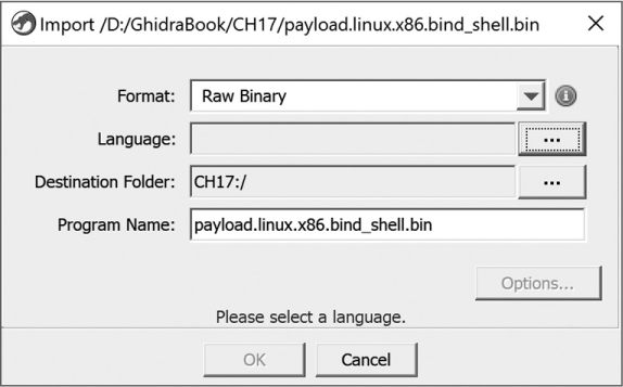
Figure 17-1: Raw Binary loader example

So what happened when we tried to import this file? Let’s start with a high-level view of Ghidra’s process for loading a file:

1. In the Ghidra Project window, the user specifies a file to load into a project.
2. The Ghidra Importer polls all of the Ghidra loaders, and each loader tries to identify the file. Each then responds with a list of load specifications to populate the Import dialog if it can load the file. (An empty list means “I can’t load this file.”)
3. The Importer collects responses from all of the loaders, builds a list of loaders that recognize the file, and presents a populated Import dialog to the user.
4. The user chooses a loader and associated information for loading the file.
5. The Importer invokes the user-selected loader that then loads the file.

For the file in Figure 17-1, none of the format-specific loaders responded with a “yes.” As a result, the task was passed to the only loader willing to take any file at any time—the Raw Binary loader. This loader performs almost no work, shifting the analysis burden to the reverse engineer. If you ever find yourself analyzing similar files that all appear to have the “raw” format, it may be time to build a specialized loader to help you with some or all of the loading process. Several tasks need to be undertaken to create a new loader that Ghidra can use to load a file in a new format.

In this chapter, we first walk you through analysis of a file whose format is not recognized by Ghidra. This will help you understand the process of analyzing an unknown file and also make a strong case for building a loader, which is how we will spend the second half of the chapter.

Unknown File Analysis

Ghidra includes loader modules to recognize many of the more common executable and archive file formats, but there is no way that Ghidra can accommodate the ever-increasing number of file formats for storing executable code. Binary images may contain executable files formatted for use with specific operating systems, ROM images extracted from embedded systems, firmware images extracted from flash updates, or simply raw blocks of machine language, perhaps extracted from network packet captures. The format of these images may be dictated by the operating system (executable files), the target processor and system architecture (ROM images), or nothing at all (exploit shellcode embedded in application layer data).

Assuming that a processor module is available to disassemble the code contained in the unknown binary, it will be your job to properly arrange the file image within Ghidra before informing Ghidra which portions of the binary represent code and which portions of the binary represent data. For most processor types, the result of loading a file using the raw format is simply a list of the contents of the file piled into a single segment, beginning at address zero, as shown in Listing 17-1.

00000000 4d       ??         4Dh    M
00000001 5a       ??         5Ah    Z
00000002 90       ??         90h
00000003 00       ??         00h
00000004 03       ??         03h
00000005 00       ??         00h
00000006 00       ??         00h
00000007 00       ??         00h

Listing 17-1: Initial lines of an unanalyzed PE file loaded using the Raw Binary loader

In some cases, depending on the sophistication of the selected processor module, some disassembly takes place. For example, a selected processor for an embedded microcontroller can make specific assumptions about the memory layout of ROM images, or an analyzer with knowledge of common code sequences associated with a specific processor can optimistically format any matches as code.

When you are faced with an unrecognized file, arm yourself with as much information about the file as you can get your hands on. Useful resources might include notes on how and where the file was obtained, processor references, operating system references, system design documentation, and any memory layout information obtained through debugging or hardware-assisted analysis (such as via logic analyzers).

In the following section, for the sake of example, we assume that Ghidra does not recognize the Windows PE file format. PE is a well-known file format that many readers may be familiar with. More importantly, documents detailing the structure of PE files are widely available, which makes dissecting an arbitrary PE file a relatively simple task.

Manually Loading a Windows PE File

When you can find documentation on the format of a particular file, your life will be significantly easier as you attempt to use Ghidra to help you make sense of the binary. Listing 17-1 shows the first few lines of an unanalyzed PE file loaded into Ghidra using the Raw Binary loader and x86:LE:32:default:windows as its language/compiler specification.¹ The PE specification states that a valid PE file begins with an MS-DOS header structure, beginning with the 2-byte signature, 4Dh 5Ah (MZ), which we see in the first two lines of Listing 17-1.² The 4-byte value located at offset 0x3C in the file contains the offset to the next header we need to find: the PE header.

Two strategies for breaking down the fields of the MS-DOS header are (1) to define appropriately sized data values for each field in the MS-DOS header and (2) to use Ghidra’s Data Type Manager functionality to define and apply an IMAGE_DOS_HEADER structure in accordance with the PE file specification. We will look at the challenges associated with option 1 in an example later in the chapter. In this case, option 2 requires significantly less effort.

When using the Raw Binary loader, Ghidra does not load the Data Type Manager with the Windows data types, so we can load the archive containing MS-DOS types, windows_vs12_32.gdt, ourselves. Locate the IMAGE_DOS_HEADER either by navigating to it within the archive or choosing CTRL-F to find it in the Data Type Manager window; then drag and drop the header onto the start of the file. You can also place the cursor on the first address in the listing and choose Data ▸ Choose Data Type (or hotkey T) from the right-click context menu and enter, or navigate to, the data type in the resulting Data Type Chooser dialog. Any of these options yields the following listing, with descriptive end-of-line comments describing each field:

00000000 4d 5a      WORD      5A4Dh    e_magic
00000002 90 00      WORD      90h      e_cblp
00000004 03 00      WORD      3h       e_cp
00000006 00 00      WORD      0h       e_crlc
00000008 04 00      WORD      4h       e_cparhdr
0000000a 00 00      WORD      0h       e_minalloc
0000000c ff ff      WORD      FFFFh    e_maxalloc
0000000e 00 00      WORD      0h       e_ss
00000010 b8 00      WORD      B8h      e_sp
00000012 00 00      WORD      0h       e_csum
00000014 00 00      WORD      0h       e_ip
00000016 00 00      WORD      0h       e_cs
00000018 40 00      WORD      40h      e_lfarlc
0000001a 00 00      WORD      0h       e_ovno
0000001c 00 00 00   WORD[4]            e_res
         00 00 00
         00 00
00000024 00 00      WORD      0h       e_oemid
00000026 00 00      WORD      0h       e_oeminfo
00000028 00 00 00   WORD[10]           e_res2
         00 00 00
         00 00 00
0000003c d8 00 00   LONG      D8h      e_lfanew

The e_lfanew field in the final line of the previous listing has a value of D8h, indicating that a PE header should be found at offset D8h (216 bytes) into the binary. Examining the bytes at offset D8h should reveal the magic number for a PE header, 50h 45h (PE), which indicates that we should apply an IMAGE_NT_HEADERS structure at offset D8h into the binary. Here is a portion of the resulting expanded Ghidra listing:

000000d8    IMAGE_NT_HEADERS
   000000d8       DWORD           4550h     Signature
   000000dc    IMAGE_FILE_HEADER            FileHeader
      000000dc    WORD            14Ch      Machine➊
      000000de    WORD            5h        NumberOfSections➋
      000000e0    DWORD           40FDFD    TimeDateStamp
      000000e4    DWORD           0h        PointerToSymbolTable
      000000e8    DWORD           0h        NumberOfSymbols
      000000ec    WORD            E0h       SizeOfOptionalHeader
      000000ee    WORD            10Fh      Characteristics
   000000f0    IMAGE_OPTIONAL_HEADER32      OptionalHeader
      000000f0    WORD            10Bh      Magic
      000000f2    BYTE            'u0006'  MajorLinkerVersion
      000000f3    BYTE            ''      MinorLinkerVersion
      000000f4    DWORD           21000h    SizeOfCode
      000000f8    DWORD           A000h     SizeOfInitializedData
      000000fc    DWORD           0h        SizeOfUninitializedData
      00000100    DWORD           14E0h     AddressOfEntryPoint➌
      00000104    DWORD           1000h     BaseOfCode
      00000108    DWORD           1000h     BaseOfData
      0000010c    DWORD           400000h   ImageBase➍
      00000110    DWORD           1000h     SectionAlignment➎
      00000114    DWORD           1000h     FileAlignment➏

At this point, we have revealed a number of interesting pieces of information that will help us to further refine the layout of the binary. First, the Machine field ➊ in a PE header indicates the target processor type for which the file was built. The value 14Ch indicates that the file is for use with x86 processor types. Had the machine type been something else, such as 1C0h (ARM), we would need to close the CodeBrowser, right-click our file in the Project window to select the Set Language option, and choose the correct language setting.

The ImageBase field ➍ indicates the base virtual address for the loaded file image. Using this information, we can incorporate some virtual address information into the CodeBrowser. Using the Window ▸ Memory Map menu option, we are shown the list of memory blocks (Figure 17-2) that make up the current program. In this case, a single memory block contains all of the program’s content. The Raw Binary loader has no means of determining appropriate memory addresses for any of our program’s content, so it places all of the content in a single memory block starting at address zero.

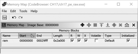
Figure 17-2: The Memory Map window

The Memory Map window’s tool buttons, shown in Figure 17-3, are used to manipulate memory blocks. In order to properly map our image into memory, the first thing we need to do is set the base address specified in the PE header.

Figure 17-3: Memory Map window tools

The ImageBase field ➍ tells us that the correct base address for this binary is 00400000. We can use the Set Image Base option to adjust the image base from the default to this value. Once we click OK, all Ghidra windows will be updated to reflect the new memory layout of the program, as shown in Figure 17-4. (Be careful using this option after you already have multiple memory blocks defined; it will shift every memory block the same distance as the base memory block.)

Figure 17-4: Memory Map after setting image base

The AddressOfEntryPoint field ➌ specifies the relative virtual address (RVA) of the program entry point. In the PE file specification, an RVA is a relative offset from the program’s base virtual address, while the program entry point is the address of the first instruction within the program file that will be executed. In this case, an entry point RVA of 14E0h indicates that the program will begin execution at virtual address 4014E0h (400000h + 14E0h). This is our first indication of where we should begin looking for code within the program. Before we can do that, however, we need to properly map the remainder of the program to appropriate virtual addresses.

The PE format uses sections to describe the mapping of file content to memory ranges. By parsing the section headers for each section in the file, we can complete the basic virtual memory layout of the program. The NumberOfSections field ➋ indicates the number of sections contained in a PE file (in this case, five). According to the PE specification, an array of section header structures immediately follows the IMAGE_NT_HEADERS structure. Individual elements in the array are IMAGE_SECTION_HEADER structures, which we define in the Ghidra structures editor and apply (five times, in this case) to the bytes following the IMAGE_NT_HEADERS structure. Alternatively, you can select the first byte of the first section header and set its type to IMAGE_SECTION_HEADER[n], where n is 5 in this example, to collapse the entire array into a single Ghidra display line.

The FileAlignment field ➏ and the SectionAlignment field ➎ indicate how the data for each section is aligned within the file and how that same data will be aligned when mapped into memory. In our example, both fields are set to align on 1000h byte offsets.³ In the PE format, there is no requirement that these two numbers be the same. The fact that they are the same does make our lives easier, however, as it means that offsets to content within the disk file are identical to offsets to the corresponding bytes in the loaded memory image of the file. Understanding how sections are aligned is important in helping us avoid errors when we manually create sections for our program.

After structuring each of the section headers, we have enough information to create additional segments within the program. Applying an IMAGE_SECTION_HEADER template to the bytes immediately following the IMAGE_NT_HEADERS structure yields the first section header in our Ghidra listing:

004001d0    IMAGE_SECTION_HEADER
   004001d0       BYTE[8]         ".text"   Name➊
   004001d8    _union_226                   Misc
      004001d8    DWORD           20A80h    PhysicalAddress
      004001d8    DWORD           20A80h    VirtualSize
   004001dc       DWORD           1000h     VirtualAddress➋
   004001e0       DWORD           21000h    SizeOfRawData➌
   004001e4       DWORD           1000h     PointerToRawData➍
   004001e8       DWORD           0h        PointerToRelocations
   004001ec       DWORD           0h        PointerToLinenumbers
   004001f0       WORD            0h        NumberOfRelocations
   004001f2       WORD            0h        NumberOfLinenumbers

The Name field ➊ informs us that this header describes the .text section. All of the remaining fields are potentially useful in formatting the listing, but we will focus on the three that describe the layout of the section. The PointerToRawData field ➍ (1000h) indicates the file offset at which the content of the section can be found. Note that this value is a multiple of the file alignment value, 1000h. Sections within a PE file are arranged in increasing file offset (and virtual address) order. Since this section begins at file offset 1000h, the first 1000h bytes of the file contain file header data and padding (if there are fewer than 1000h bytes of header data, the section must be padded to a 1000h byte boundary). Therefore, even though the header bytes do not, strictly speaking, constitute a section, we can highlight the fact that they are logically related by grouping them into a memory block in the Ghidra listing.

Ghidra offers two ways to create new memory blocks, both accessed through the Memory Map window from Figure 17-2. The Add Block tool (refer to Figure 17-3) opens the dialog shown in Figure 17-5, which is used to add new memory blocks that do not overlap with any existing memory block. The dialog asks for the name of the new memory block, its start address, and its length. The block may be initialized with a constant value (zero-filled, for example), initialized with content from the current file (you indicate the file offset from which the content is taken), or left uninitialized.

The second way to create a new block is to split an existing block. To split a block in Ghidra, you must first select the block to split in the Memory Map window and then use the Split Block tool (refer to Figure 17-3) to open the dialog shown in Figure 17-6. We are just starting out, so we have only one block to split. We start by splitting the file at the beginning of the .text section to carve the program headers off of the beginning of the existing block. When we enter the length (1000h) of our block to split (the header section), Ghidra automatically computes the remaining address and length fields. All that is left is to provide a name for the new block being created at the split point. Here, we use the name contained in the first section header: .text.

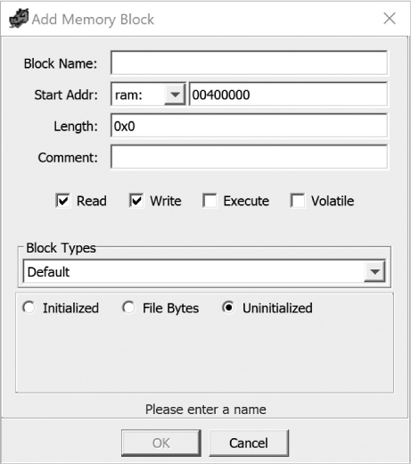
Figure 17-5: The Add Memory Block dialog

Figure 17-6: The Split Block dialog

We now have two blocks in our memory map. The first block contains the correctly sized program headers. The second block contains the correctly named, but not correctly sized, .text section. This situation is reflected in Figure 17-7, where we can see that the size of the .text section is 0x29000 bytes.

Figure 17-7: Memory Map window after splitting a block

Returning to the header for the .text section, we see that the VirtualAddress field ➋ (1000h) is an RVA that specifies the memory offset (from ImageBase) at which the section content begins and that the SizeOfRawData field ➌ (21000h) indicates how many bytes of data are present in the file. In other words, this particular section header tells us that the .text section is created by mapping the 21000h bytes from file offsets 1000h-21FFFh to virtual addresses 401000h-421FFFh.

Because we split the original memory block at the beginning of the .text section, the newly created .text section temporarily contains all remaining sections, since its current size of 0x29000 is greater than the correct size of 0x21000. By consulting the remaining section headers and repeatedly splitting the last memory block, we make progress toward a correct final memory map for the program. However, a problem arises when we reach the following pair of section headers:

00400220    IMAGE_SECTION_HEADER
   00400220       BYTE[8]         ".data"   Name
   00400228    _union_226                   Misc
      00400228    DWORD           5624h     PhysicalAddress
      00400228    DWORD           5624h     VirtualSize➊
   0040022c       DWORD           24000h    VirtualAddress➋
   00400230       DWORD           4000h     SizeOfRawData➌
   00400234       DWORD           24000h    PointerToRawData
   00400238       DWORD           0h        PointerToRelocations
   0040023c       DWORD           0h        PointerToLinenumbers
   00400240       WORD            0h        NumberOfRelocations
   00400242       WORD            0h        NumberOfLinenumbers
   00400244       DWORD           C0000040h Characteristics
00400248    IMAGE_SECTION_HEADER
   00400248       BYTE[8] ".idata" Name
   00400250    _union_226 Misc
      00400250    DWORD           75Ch      PhysicalAddress
      00400250    DWORD           75Ch      VirtualSize
   00400254       DWORD           2A000h    VirtualAddress➍
   00400258       DWORD           1000h     SizeOfRawData
   0040025c       DWORD           28000h    PointerToRawData➎
   00400260       DWORD           0h        PointerToRelocations
   00400264       DWORD           0h        PointerToLinenumbers
   00400268       WORD            0h        NumberOfRelocations
   0040026a       WORD            0h        NumberOfLinenumbers
   0040026c       DWORD           C0000040h Characteristics

The .data section’s virtual size ➊ is larger than its file size ➌. What does this mean and how does it impact our memory map? The compiler has concluded that the program requires 5624h bytes of runtime static data, but supplies only 4000h bytes to initialize that data. The remaining 1624h bytes of runtime data will not be initialized with content from the executable file, as they are allocated for uninitialized global variables. (It is not uncommon to see such variables allocated within a dedicated program section named .bss.)

To finalize our memory map, we must choose an appropriate size for the .data section and ensure that subsequent sections are correctly mapped as well. The .data section maps 4000h bytes of file data from file offset 24000h to memory address 424000h ➋ (ImageBase + VirtualAddress). The next section (.idata) maps 1000h bytes from file offset 28000h ➎ to memory address 42A000h ➍. If you’re paying close attention, you may have noticed that the .data section appears to occupy 6000h bytes in memory (42A000h–424000h), and in fact it does. The reasoning behind this size is that the .data section requires 5624h bytes, but this is not an even multiple of 1000h, so the section will be padded up to 6000h bytes so that the .idata section properly adheres to the section alignment requirement specified in the PE header. In order to finish our memory map, we must carry out the following actions:

1. Split the .data section using a length of 4000h. The resulting .idata section will, for the moment, start at 428000h.
2. Move the .idata section to address 42A000h by clicking the Move Block icon (Figure 17-3) and setting the start address to 42A000h.
3. Split off, and, if necessary, move any remaining sections to achieve the final program layout.
4. Optionally, expand any sections whose virtual size aligns to a higher boundary than their file size. In our example, the .data section’s virtual size, 5624h, aligns to 6000h, while its file size, 4000h, aligns to 4000h. Once we have created room by moving the .idata section to its proper location, we will expand the .data section from 4000h to 6000h bytes.

To expand the .data section, highlight the .data section in the Memory Map window and then select the Expand Down tool (refer to Figure 17-3) to modify the end address (or length) of the section. The Expand Block Down dialog is shown in Figure 17-8. (This operation will add the .exp extension to the section name.)

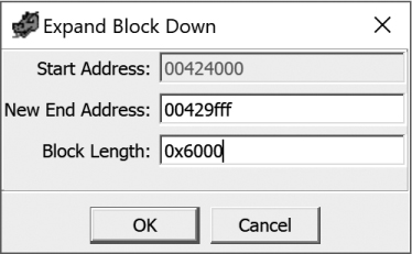
Figure 17-8: The Expand Block Down dialog

Our final memory map, obtained after the series of block moves, splits, and expansions, appears in Figure 17-9. In addition to the section name, start and end addresses, and length columns, read (R), write (W), and execute (X) permissions are shown for each section in the form of checkboxes. For PE files, these values are specified via bits in the Characteristics field of each section header. Consult the PE specification for information on parsing the Characteristics field to properly set permissions for each section.

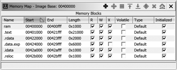
Figure 17-9: Final Memory Map window after creating all sections

With all program sections properly mapped, we need to locate some bytes that have a high likelihood of being code. The AddressOfEntryPoint (RVA 14E0h, or virtual address 4014E0h) leads us to the program’s entry point, which is known to be code. Navigating to this location, we see the following raw byte listing:

004014e0  ??     55h    U
004014e1  ??     8Bh
004014e2  ??     ECh
...

Using the context menu to disassemble (hotkey D) from address 004014e0 starts the recursive descent process (whose progress may be tracked in the lower-right corner of the Code Browser) and causes the bytes above to be reformatted as the code seen here:

     FUN_004014e0
004014e0  PUSH   EBP
004014e1  MOV    EBP,ESP
004014e3  PUSH   -0x1
004014e5  PUSH   DAT_004221b8
004014ea  PUSH   LAB_004065f0
004014ef  MOV    EAX,FS:[0x0]
004014f5  PUSH   EAX

At this point, we would hope that we had enough code to perform a comprehensive analysis of the binary. If we had fewer clues regarding the memory layout of the binary, or the separation between code and data within the file, we would need to rely on other sources of information to guide our analysis. Some potential approaches to determining correct memory layout and locating code include the following:

• Use processor reference manuals to understand where reset vectors may be found.
• Search for strings in the binary that might suggest the architecture, operating system, or compiler used to build the binary.
• Search for common code sequences such as function prologues associated with the processor for which the binary was built.
• Perform statistical analysis over portions of the binary to find regions that look statistically similar to known binaries.
• Look for repetitive data sequences that might be tables of addresses (for example, many nontrivial 32-bit integers that all share the same upper 12 bits).⁴ These may be pointers and may provide clues regarding the memory layout of the binary.

In rounding out our discussion of loading raw binaries, consider that you would need to repeat each step covered in this section every time you open a binary with the same format that remains unknown to Ghidra. Along the way, you might automate some of your actions by writing scripts that perform some of the header parsing and segment creation for you. This is exactly the purpose of a Ghidra loader module! In the next section, we’ll write a simple loader module to introduce Ghidra’s loader module architecture, before moving on to more sophisticated loader modules that perform some common tasks associated with loading files that adhere to a structured format.

Example 1: SimpleShellcode Loader Module

At the beginning of this chapter, we tried to load a shellcode file into Ghidra and were referred to the Raw Binary loader. In Chapter 15, we used Eclipse and GhidraDev to create an analyzer module and then added it as an extension to Ghidra. Recall that one of the module options provided by Ghidra was to create a loader module. In this chapter, we will build a simple loader module as an extension to Ghidra to load shellcode. As in our Chapter 15 example, we will use a simplified software development process, as this is just a simple demonstration project. Our process will include the following steps:

1. Define the problem.
2. Create the Eclipse module.
3. Build the loader.
4. Add the loader to our Ghidra installation.
5. Test the loader from our Ghidra installation.

Step 0: Take a Step Back

Before we can even start to define the problem, we need to understand (a) what Ghidra currently does with a shellcode file and (b) what we would like Ghidra to do with a shellcode file. Basically, we have to load and analyze a shellcode file as a raw binary and then use the information we discover to inform the development of our shellcode loader (and potentially an analyzer). Fortunately for us, most shellcode is not nearly as complicated as a PE file. Let’s take a deep breath and dive into the world of shellcode.

Let’s start by analyzing the shellcode file we tried to load at the beginning of the chapter. We loaded the file and were referred to the Raw Binary loader as our only option, as shown earlier in Figure 17-1. There was no recommendation for a language as the Raw Binary loader just “inherited” our file because none of the other loaders wanted it. Let’s select a relatively common language/compiler specification, x86:LE:32:default:gcc, as shown in Figure 17-10.

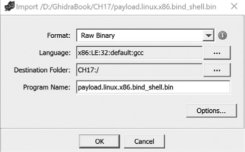
Figure 17-10: Import dialog with language/compiler specification

We click OK and get an Import Results Summary window that includes the content shown in Figure 17-11.

Figure 17-11: Import Results Summary for shellcode file

Based on the contents of the enlarged block in the summary, we know that there are only 78 bytes in the file in one memory/data block, and that is about all the help we get from the Raw Binary loader. If we open the file in the CodeBrowser, Ghidra will offer to auto analyze the file. Regardless of whether or not Ghidra auto analyzes the file, the Listing window in the CodeBrowser displays the content shown in Figure 17-12. Note that there is only one section in Program Trees, the Symbol Tree is empty, and the Data Type Manager has no entries in the folder specific to the file. In addition, the Decompiler window remains empty, as no functions have been identified in the file.

Figure 17-12: CodeBrowser window after loading (or analyzing) the shellcode file

Right-click the first address in the file and choose Disassemble (hotkey D) from the context menu. In the Listing window, we now see something we can work with—a list of instructions! Listing 17-2 shows the instructions after disassembly and after we have done some analysis on the file. The end-of-line comments document some of the analysis of this short file.

0000002b  INC    EBX
0000002c  MOV    AL,0x66       ; 0x66 is Linux sys_socketcall
0000002e  INT    0x80          ; transfers flow to kernel to
                               ; execute system call
00000030  XCHG   EAX,EBX
00000031  POP    ECX
        LAB_00000032             XREF[1]:  00000038(j)
00000032  PUSH   0x3f          ; 0x3f is Linux sys_dup2
00000034  POP    EAX
00000035  INT    0x80          ; transfers flow to kernel to
                               ; execute system call
00000037  DEC    ECX
00000038  JNS   LAB_00000
0000003a  PUSH   0x68732f2f    ; 0x68732f2f converts to "//sh"
0000003f  PUSH   0x6e69622f    ; 0x6e69622f converts to "/bin"
00000044  MOV    EBX,ESP
00000046  PUSH   EAX
00000047  PUSH   EBX
00000048  MOV    ECX,ESP
0000004a  MOV    AL,0xb        ; 0xb is Linux sys_execve which
                               ; executes a specified program
0000004c  INT    0x80          ; transfers flow to kernel to
                                      ; execute system call

Listing 17-2: Disassembled 32-bit Linux shellcode

Based on our analysis, the shellcode invokes the Linux execve system call (at 0000004c) to launch /bin/sh (which was pushed onto the stack at 0000003a and 000003f). The fact that these instructions have meaning to us indicates that we likely chose an appropriate language and disassembly starting point.

We now know enough about the loading process to define our loader. (We also have enough information to build a simple shellcode analyzer, but that is a task for another day.)

Step 1: Define the Problem

Our task is to design and develop a simple loader that will load shellcode into our Listing window and set the entry point, which will facilitate auto analysis. The loader needs to be added to Ghidra and be available as a Ghidra Loader option. It also needs to be able to respond to the Ghidra Importer poll in an appropriate manner: the same way as the Raw Binary loader does. This will make our new loader a second catchall loader option. As a side note, all of the examples will utilize the FlatProgramAPI. While the FlatProgramAPI is not generally used for building extensions, its use will reinforce the scripting concepts presented in Chapter 14 that you are likely to use when developing Ghidra scripts in Java.

Step 2: Create the Eclipse Module

As discussed in Chapter 15, use GhidraDev ▸ New ▸ Ghidra Module Project to create a module called SimpleShellcode that uses the Loader Module template. This will create a file called SimpleShellcodeLoader.java in the src/main/java folder within the SimpleShellcode module. This folder hierarchy is shown in context in Figure 17-13.

Figure 17-13: SimpleShellcode hierarchy

Step 3: Build the Loader

A partial image of the loader template SimpleShellcodeLoader.java is shown in Figure 17-14. The functions have been collapsed so that you can see all of the loader methods provided in the loader template. Recall that Eclipse will recommend imports if you need them as you develop your code, so you can jump right into coding and accept the recommended import statements when Eclipse detects that you need them.

Figure 17-14: SimpleShellcodeLoader template

Within the loader template in Figure 17-14 are six task tags to the left of the line numbers that indicate where you should start your development. We will expand each section as we address specific tasks and include the before and after content associated with each task so you will understand how you need to modify the template. (Some content will be wrapped or reformatted for readability and comments minimized to conserve space.) Unlike the analyzer module you wrote in Chapter 15, this module does not require any obvious class member variables, so you can jump right into the tasks at hand.

Step 3-1: Document the Class

When you expand the first task tag, you see the following task description:

/**
 * TODO: Provide class-level documentation that describes what this
 * loader does.
 */

This task involves replacing the existing TODO comments with comments that describe what the loader does:

/*
 * This loader loads shellcode binaries into Ghidra,
 * including setting an entry point.
 */

Step 3-2: Name and Describe the Loader

Expanding the next task tag reveals a TODO comment and the string you need to edit. This makes it easy to identify where you should start working. The second task contains the following:

public String getName() {
       // TODO: Name the loader.  This name must match the name
       // of the loader in the .opinion files
     return "My loader"➊;
}

Change the string ➊ to something meaningful. You don’t need to worry about matching the name in the .opinion files, as they are not applicable to loaders that will accept any files. You will see .opinion files when you get to the third example. Ignoring the .opinion file comment in the template results in the following code:

public String getName() {
   return "Simple Shellcode Loader";
}

Step 3-3: Determine If the Loader Can Load This File

The second step in the loading process we described at the beginning of the chapter involved the Importer loader poll. This task requires you to determine if your loader can load the file and provide a response to the Importer through your method’s return value:

public Collection<LoadSpec> findSupportedLoadSpecs(ByteProvider provider)
                            throws IOException {
   List<LoadSpec> loadSpecs = new ArrayList<>();

   // TODO: Examine the bytes in 'provider' to determine if this loader
   // can load it.  If it can load it, return the appropriate load
   // specifications.
   return loadSpecs;
}

Most loaders do this by examining the content of the file to find a magic number or header structure. The ByteProvider input parameter is a Ghidra-provided read-only wrapper around an input file stream. We are going to simplify our task and adopt the LoadSpec list that the Raw Binary loader uses, which ignores file content and simply lists all possible LoadSpecs. We will then give our loader a lower priority than the Raw Binary loader so that if a more specific loader exists, it will automatically have a higher priority in the Ghidra Import dialog.

public Collection<LoadSpec> findSupportedLoadSpecs(ByteProvider provider)
                                                   throws IOException {
   // The List of load specs supported by this loader
   List<LoadSpec> loadSpecs = new ArrayList<>();
   List<LanguageDescription> languageDescriptions =
        getLanguageService().getLanguageDescriptions(false);
   for (LanguageDescription languageDescription : languageDescriptions) {
      Collection<CompilerSpecDescription> compilerSpecDescriptions =
         languageDescription.getCompatibleCompilerSpecDescriptions();
      for (CompilerSpecDescription compilerSpecDescription :
           compilerSpecDescriptions) {
         LanguageCompilerSpecPair lcs =
            new LanguageCompilerSpecPair(languageDescription.getLanguageID(),
            compilerSpecDescription.getCompilerSpecID());
         loadSpecs.add(new LoadSpec(this, 0, lcs, false));
      }
   }
   return loadSpecs;
}

Every loader has an associated tier and tier priority. Ghidra defines four tiers of loaders, ranging from highly specialized (tier 0) to format agnostic (tier 3). When multiple loaders are willing to accept a file, Ghidra sorts the loader list displayed to the user in increasing tier order. Loaders within the same tier are further sorted in increasing tier priority order (that is, tier priority 10 is listed before tier priority 20).

For example, the PE loader and the Raw Binary loader are both willing to load PE files, but the PE loader is a better choice to load this format (its tier is 1), so it will appear before the Raw Binary loader (tier 3, tier priority 100) in the list. We set the Simple Shellcode Loader’s tier to 3 (LoaderTier.UNTARGETED_LOADER) and priority to 101, so it will be given the lowest priority by the Importer when populating the Import window with candidate loaders. To accomplish this, add the following two methods to your loader:

@Override
public LoaderTier getTier() {
   return LoaderTier.UNTARGETED_LOADER;
}
@Override
public int getTierPriority() {
   return 101;
}

Step 3-4: Load the Bytes

The following method shown before and after we edit the content does the heavy lifting of loading content from the file being imported into our Ghidra project (in this case, it loads the shellcode):

protected void load(ByteProvider provider, LoadSpec loadSpec,
               List<Option> options, Program program, TaskMonitor monitor,
               MessageLog log) throws CancelledException, IOException {

   // TODO: Load the bytes from 'provider' into the 'program'.
}

protected void load(ByteProvider provider, LoadSpec loadSpec,
               List<Option> options, Program program, TaskMonitor monitor,
               MessageLog log) throws CancelledException, IOException {
➊ FlatProgramAPI flatAPI = new FlatProgramAPI(program);
   try {
      monitor.setMessage("Simple Shellcode: Starting loading");
      // create the memory block we're going to load the shellcode into
      Address start_addr = flatAPI.toAddr(0x0);
   ➋ MemoryBlock block = flatAPI.createMemoryBlock("SHELLCODE",
      start_addr, provider.readBytes(0, provider.length()), false);
      // make this memory block read/execute but not writeable
   ➌ block.setRead(true);
      block.setWrite(false);
      block.setExecute(true);
      // set the entry point for the shellcode to the start address
   ➍ flatAPI.addEntryPoint(start_addr);
      monitor.setMessage( "Simple Shellcode: Completed loading" );
   } catch (Exception e) {
      e.printStackTrace();
      throw new IOException("Failed to load shellcode");
   }
}

Note that, unlike the scripts in Chapters 14 and 15, which inherit from GhidraScript (and ultimately FlatProgramAPI), our loader class has no direct access to the Flat API. Therefore, to simplify our access to some commonly used API classes, we instantiate our own FlatProgramAPI object ➊. Next, we create a MemoryBlock named SHELLCODE at address zero ➋ and populate it with the entire contents of the input file. We take the time to set some reasonable permissions ➌ on the new memory region before adding an entry point ➍ that informs Ghidra where it should begin its disassembly.

Adding an entry point is a very important step for a loader. The presence of entry points is the primary means by which Ghidra locates addresses known to contain code (as opposed to data). As it parses the input file, the loader is ideally suited to discover any entry points and identify them to Ghidra.

Step 3-5: Register Custom Loader Options

Some loaders offer users the option to modify various parameters associated with the loading process. You may override the getDefaultOptions function to provide Ghidra with a list of custom options available for your loader:

public List<Option> getDefaultOptions(ByteProvider provider, LoadSpec
       loadSpec,DomainObject domainObject, boolean isLoadIntoProgram) {
   List<Option> list = super.getDefaultOptions(provider, loadSpec,

                       domainObject, isLoadIntoProgram);
   // TODO: If this loader has custom options, add them to 'list'
   list.add(new Option("Option name goes here",
                        Default option value goes here));
   return list;
}

Since this loader is just for demonstration purposes, we will not add any options. Options for a loader might include setting an offset into the file at which to start reading, and setting the base address at which to load the binary. To view the options associated with any loader, click the Options . . . button on the bottom right of the Import dialog (refer to Figure 17-1).

public List<Option> getDefaultOptions(ByteProvider provider, LoadSpec
       loadSpec,DomainObject domainObject, boolean isLoadIntoProgram) {
   // no options
   List<Option> list = new ArrayList<Option>();
   return list;
}

Step 3-6: Validate Options

The next task is to validate the options:

public String validateOptions(ByteProvider provider, LoadSpec loadSpec,
                              List<Option> options, Program program) {

   // TODO: If this loader has custom options, validate them here.
   // Not all options require validation.
   return super.validateOptions(provider, loadSpec, options, program);
}

As we do not have any options, we just return null:

public String validateOptions(ByteProvider provider, LoadSpec loadSpec,
                              List<Option> options, Program program) {

   // No options, so no need to validate
   return null;
}

Step 4: Add the Loader to Our Ghidra Installation

After confirming that this module functions correctly, export the Ghidra module extension from Eclipse and then install the extension in Ghidra, just as we did with the SimpleROPAnalyzer module in Chapter 15. Select GhidraDev ▸ Export ▸ Ghidra Module Extension, choosing the SimpleShellcode module, and follow the same click-through process that you did in Chapter 15.

To import the extension into Ghidra, choose File ▸ Install Extensions from the Ghidra Project window. Add the new loader to the list and select it. Once you restart Ghidra, the new loader should be available as an option, but you should test to be sure.

Step 5: Test the Loader Within Ghidra

Our simplified test plan is just to demonstrate functionality. SimpleShellcode passed an acceptance test consisting of the following criteria:

1. (Pass) SimpleShellcode appears as a loader option with lower priority than Raw Binary.
2. (Pass) SimpleShellcode loads a file and sets the entry point.

Test case 1 passed, as shown in Figure 17-15. A second confirmation is shown in Figure 17-16, where the PE file analyzed earlier in the chapter is being loaded. In both cases, we see that the Simple Shellcode Loader option has the lowest priority in the Format list.

Figure 17-15: Import window with our new loader listed as an option

Figure 17-16: Import window with our new loader listed as an option for a PE file

Choose the language specification based on the information available about the binary and how it was obtained. Let’s assume that the shellcode was captured from packets headed for an x86 box. In that case, selecting x86:LE:32:default:gcc for our language/compiler specification is probably a good starting point.

After we select a language and click OK for the file shown in Figure 17-15, the binary will be imported into our Ghidra project. We can then open the program in the CodeBrowser, and Ghidra will provide us an option to analyze the file. If we accept the analysis, we will see the following listing:

     undefined FUN_00000000()
        undefined  AL:1 <RETURN>
        undefined4 Stack[-0x10]:4 local_10  XREF[1]: 00000022(W)
     FUN_00000000                           XREF[1]: Entry Point(*)➊
00000000 31 db          XOR    EBX,EBX
00000002 f7 e3          MUL    EBX
00000004 53             PUSH   EBX
00000005 43             INC    EBX
00000006 53             PUSH   EBX
00000007 6a 02          PUSH   0x2
00000009 89 e1          MOV    ECX,ESP
0000000b b0 66          MOV    AL,0x66
0000000d cd 80          INT    0x80
0000000f 5b             POP    EBX
00000010 5e             POP    ESI
00000011 52             PUSH   EDX
00000012 68 02 00 11 5c PUSH   0x5c110002

An entry point ➊ is identified, so Ghidra is able to provide us with a disassembly to begin our analysis.

SimpleShellcodeLoader was a trivial example, as shellcode is generally found embedded within some other data. For demonstration purposes, we will use our loader module as a base to create a loader module that extracts shellcode from C source files and loads the shellcode for analysis. This may, for example, allow us to build shellcode signatures that Ghidra can recognize in other binaries. We will not go into great depth for each step, as we are just augmenting the capabilities of our existing shellcode loader.

Example 2: Simple Shellcode Source Loader

Since modules provide a way to organize code, and the SimpleShellcode module you created has everything required to create a loader, you don’t need to create a new module. Simply choose File ▸ New ▸ File from the Eclipse menu and add a new file (SimpleShellcodeSourceLoader.java) to your SimpleShellcode src/main/java folder. By doing this, all of your new loaders will be included in your new Ghidra extension.

To make life simple, paste the contents of your existing SimpleShellcodeLoader.java into this new file and update the comments about what the loader does. The following steps highlight the parts of the existing loader that you need to change to make the new loader work as expected. For the most part, you will be adding onto the existing code.

Update 1: Modify the Response to the Importer Poll

The simple source loader is going to make its decision based strictly on the file extension. If the file does not end in .c, the loader will return an empty loadSpecs list. If the file does end with .c, it will return the same loadSpecs list that it did for the previous loader. To make this work, you need to add the following test to the findSupportLoadSpecs method:

// The List of load specs supported by this loader
List<LoadSpec> loadSpecs = new ArrayList<>();
// Activate loader if the filename ends in a .c extension
if (!provider.getName().endsWith(".c")) {
   return loadSpecs;
}

We’ve also decided that our loader deserves a higher priority than the Raw Binary loader because ours identifies a particular type of file to accept and is better suited for that type of file. This is done by returning a higher priority (lower value) from our getTierPriority method:

public int getTierPriority() {
   // priority of this loader
   return 99;
}

Update 2: Find the Shellcode in the Source Code

Recall that shellcode is just raw machine code that does something useful for us. The individual bytes in the shellcode will lie in the range 0..255, and many of these values fall outside the range of ASCII printable characters. Therefore, when shellcode is embedded into a source file, much of it must be represented using hex escape sequences such as xFF. Strings of this sort are rather unique, and we can build a regular expression to help our loader identify them. The following instance variable declaration describes the regular expression that all of the functions in our loader may use to find shellcode bytes with the selected C file:

private String pattern = "\\x[0-9a-fA-F]{1,2}";

Within the load method, the loader parses the file looking for patterns that match the regular expression to help calculate the amount of memory needed when loading the file into Ghidra. As shellcode is frequently not contiguous, the loader should parse the entire file looking for shellcode regions to load from the file.

// set up the regex matcher
CharSequence provider_char_seq =
      new String(provider.readBytes(0, provider.length())➊, "UTF-8");
Pattern p = Pattern.compile(pattern);
Matcher m = p.matcher(provider_char_seq)➋;
// Determine how many matches (shellcode bytes) were found so that we can
// correctly size the memory region, then reset the matcher
int match_count = 0;
while (m.find()) {
 ➌ match_count++;
}
m.reset();

After loading the entire contents of the input file ➊, we count all of the matches ➌ against our regular expression ➋.

Update 3: Convert Shellcode to Byte Values

The load() method next needs to convert the hex escape sequences into byte values and put them in a byte array:

byte[] shellcode = new byte[match_count];
// convert the hex representation of bytes in the source code to actual
// byte values in the binary we're creating in Ghidra
int ii = 0;
while (m.find()) {
   // strip out the x
   String hex_digits = m.group().replaceAll("[^0-9a-fA-F]+", "")➊;
   // parse what's left into an integer and cast it to a byte, then
   // set current byte in byte array to that value
   shellcode[ii++]➋ = (byte)Integer.parseInt(hex_digits, 16)➌;
}

The hex digits are extracted from each matching string ➊ and converted into byte values ➌ that get appended to our shellcode array ➋.

Update 4: Load Converted Byte Array

Finally, because the shellcode is in a byte array, the load() method needs to copy it from the byte array into the program’s memory. This is the actual loading step and the last required step for your loader to accomplish the goal:

// create the memory block and populate it with the shellcode
Address start_addr = flatAPI.toAddr(0x0);
MemoryBlock block =
      flatAPI.createMemoryBlock("SHELLCODE", start_addr, shellcode, false);

Results

To test our new loader, we create a C source file that contains the following escaped representation of x86 shellcode:

unsigned char buf[] =
   "x31xdbxf7xe3x53x43x53x6ax02x89xe1xb0x66xcdx80"
   "x5bx5ex52x68x02x00x11x5cx6ax10x51x50x89xe1x6a"
   "x66x58xcdx80x89x41x04xb3x04xb0x66xcdx80x43xb0"
   "x66xcdx80x93x59x6ax3fx58xcdx80x49x79xf8x68x2f"
   "x2fx73x68x68x2fx62x69x6ex89xe3x50x53x89xe1xb0"
   "x0bxcdx80";

Because our source file’s name ends in .c, our loader appears in the list as the top selection, with higher priority than the Raw Binary and Simple Shellcode loaders, as shown in Figure 17-17.

Figure 17-17: Import dialog for shellcode source file

Selecting this loader, using the same default compiler/language specification as the previous example (x86:LE:32:default:gcc), and letting Ghidra auto analyze the file yields the following function in the disassembly listing:

     **************************************************************
     *                         FUNCTION                           *
     **************************************************************
     undefined FUN_00000000()
        undefined AL:1 <RETURN>
        undefined4 Stack[-0x10]:4 local_10
     FUN_00000000                      XREF[1]: Entry Point(*)
00000000  XOR    EBX,EBX
00000002  MUL    EBX
00000004  PUSH   EBX
00000005  INC    EBX
00000006  PUSH   EBX

Scrolling down through the listing leads us to the familiar content (see Listing 17-2) shown here (with comments added for clarity):

        LAB_00000032
00000032  PUSH   0x3f
00000034  POP    EAX
00000035  INT    0x80
00000037  DEC    ECX
00000038  JNS    LAB_00000
0000003a  PUSH   0x68732f2f          ; 0x68732f2f converts to "//sh"
0000003f  PUSH   0x6e69622f          ; 0x6e69622f converts to "/bin"

Most reverse engineering efforts focus on binaries. In this case, we have stepped outside that box and used Ghidra to load shellcode for analysis as well as to extract shellcode from C source files. Our goal was to demonstrate the flexibility and simplicity of creating loaders for Ghidra. Now, let’s step back into that box and create a loader for a structured file format.

Assume that our target shellcode is contained within an ELF binary and that, for the sake of this example, Ghidra does not recognize ELF binaries. Further, none of us have ever heard of an ELF binary. Let the adventure begin.

Example 3: Simple ELF Shellcode Loader

Congratulations! You are now the resident RE expert on shellcode, and colleagues are reporting what they suspect is shellcode contained in binaries and are being referred by Ghidra to the Raw Binary loader. Since this does not appear to be a one-off problem, and you think there is a good chance you will see more binaries with similar characteristics, you decide to build a loader that will handle this new type of file. As discussed in Chapter 13, you can use tools internal or external to Ghidra to capture information about the file. If you once again turn to the command line, file provides helpful information to start building your loader:

$ file elf_shellcode_min
  elf_shellcode_min: ELF 32-bit LSB executable, Intel 80386, version 1 (SYSV),
  statically linked, corrupted section header size
$

The file command provides information about a format you have never heard of before, ELF. Your first step is to do some research to see if you can locate any information about this type of binary. Your friend Google will happily point you to several references about the ELF format, which you can use to locate the information you need to build your loader. Anything that provides enough accurate information to solve the problem works.⁵

As this is a bigger challenge than the previous two loader examples, we will break this into sections associated with the individual files within your Eclipse SimpleShellcode module that you will need to create/modify/delete to complete your new SimpleELFShellcodeLoader. We will start off with some simple housekeeping.

Housekeeping

The first step is to create a SimpleELFShellcodeLoader.java file within the SimpleShellcode module in Eclipse. As you don’t want to start from nothing, you should use Save As with SimpleShellcodeLoader.java to create this new file. Once you have done this, there are a few minor modifications to make to the new file before you can start focusing on the new challenge:

• Change the name of the class to SimpleELFShellcodeLoader.
• Modify the getTier method return value from UNTARGETED_LOADER to GENERIC_TARGET_LOADER.
• Delete the getTierPriority method.
• Modify the getName method to return "Simple ELF Shellcode Loader".

Once you have completed the housekeeping tasks, let’s apply the information you learned from your research about the new header format.

ELF Header Format

While researching this new format, you discover that the ELF format contains three types of headers: the file header (or ELF header), the program header(s), and the section header(s). You can start by focusing on the ELF header. Associated with each field in the ELF header is an offset as well as other information about the field. Since you need to access only a few of these fields and you won’t be modifying the offsets, declare the following constants as instance variables within your loader class to help your loader correctly parse this new header format:

private final byte[] ELF_MAGIC            = {0x7f, 0x45, 0x4c, 0x46};
private final long EH_MAGIC_OFFSET        = 0x00;
private final long EH_MAGIC_LEN           = 4;

private final long EH_CLASS_OFFSET        = 0x04;
private final byte EH_CLASS_32BIT         = 0x01;

private final long EH_DATA_OFFSET         = 0x05;
private final byte EH_DATA_LITTLE_ENDIAN  = 0x01;

private final long EH_ETYPE_OFFSET        = 0x10;
private final long EH_ETYPE_LEN           = 0x02;
private final short EH_ETYPE_EXEC         = 0x02;

private final long EH_EMACHINE_OFFSET     = 0x12;
private final long EH_EMACHINE_LEN        = 0x02;
private final short EH_EMACHINE_X86       = 0x03;

private final long EH_EFLAGS_OFFSET       = 0x24;
private final long EN_EFLAGS_LEN          = 4;

private final long EH_EEHSIZE_OFFSET      = 0x28;
private final long EH_PHENTSIZE_OFFSET    = 0x2A;
private final long EH_PHNUM_OFFSET        = 0x2C;

With a description of the ELF header in hand, the next step is to determine how to respond to the Importer poll to ensure that the new ELF loader is capable of loading only files that adhere to the ELF format. In the previous two examples, the shellcode loaders did not look at file contents to determine if they could load a file. This simplified coding these examples significantly. Now things are a bit more complicated. Fortunately, the ELF documentation provides important clues to help determine the appropriate loader specifications.

Find Supported Load Specifications

The loader can’t load anything that isn’t in the right format and can reject any file by returning an empty loadSpecs list. Within the findSupportedLoadSpecs() method, immediately eliminate all binaries that don’t have the expected magic number by using the following code:

byte[] magic = provider.readBytes(EH_MAGIC_OFFSET, EH_MAGIC_LEN);
if (!Arrays.equals(magic, ELF_MAGIC)) {
   // the binary is not an ELF
   return loadSpecs;
}

Once the undesirables have been eliminated, the loader can check the bit width and endianness to see if the architecture is reasonable for an ELF binary. For this demonstration, let’s further limit the types of binaries the loader will accept to 32-bit little-endian:

byte ei_class = provider.readByte(EH_CLASS_OFFSET);
byte ei_data = provider.readByte(EH_DATA_OFFSET);
if ((ei_class != EH_CLASS_32BIT) || (ei_data != EH_DATA_LITTLE_ENDIAN)) {
   // not an ELF we want to accept
   return loadSpecs;
}

To round out the verification process, the following code checks if this is an ELF executable file (as opposed to a shared library) for the x86 architecture:

byte[] etyp = provider.readBytes(EH_ETYPE_OFFSET, EH_ETYPE_LEN);
short e_type =
      ByteBuffer.wrap(etyp).order(ByteOrder.LITTLE_ENDIAN).getShort();
byte[] emach = provider.readBytes(EH_EMACHINE_OFFSET, EH_EMACHINE_LEN);
short e_machine =
      ByteBuffer.wrap(emach).order(ByteOrder.LITTLE_ENDIAN).getShort();
if ((e_type != EH_ETYPE_EXEC) || (e_machine != EH_EMACHINE_X86)) {
   // not an ELF we want to accept
   return loadSpecs;
}

Now that you have limited your file types, you can query the opinion service for matching language and compiler specifications. Conceptually, you query the opinion services with values extracted from the file you are loading (for example, the ELF header e_machine field), and in response you receive a list of language/compiler specifications that your loader is willing to accept. (The “behind the scenes” actions that take place when you query the opinion service are described in more detail in the following sections.)

byte[] eflag = provider.readBytes(EH_EFLAGS_OFFSET, EN_EFLAGS_LEN);
int e_flags = ByteBuffer.wrap(eflag).order(ByteOrder.LITTLE_ENDIAN).getInt();
List<QueryResult> results =
     QueryOpinionService.query(getName(), Short.toString(e_machine),
                               Integer.toString(e_flags));

Let’s assume that the opinion service is likely to yield more results than you want to handle with this loader. You can pare the list further by excluding results based on the attributes specified in the associated language/compiler specifications. The following code filters out a compiler and a processor variant:

for (QueryResult result : results) {
   CompilerSpecID cspec = result.pair.getCompilerSpec().getCompilerSpecID();
   if (cspec.toString().equals("borlanddelphi"➊)) {
      // ignore anything created by Delphi
      continue;
   }
   String variant = result.pair.getLanguageDescription().getVariant();
   if (variant.equals("System Management Mode"➋)) {
       // ignore anything where the variant is "System Management Mode"
       continue;
   }
   // valid load spec, so add it to the list
 ➌ loadSpecs.add(new LoadSpec(this, 0, result));
}
return loadSpecs;

The above examples (which you are free to include in your loader) specifically exclude the Delphi compiler ➊ and x86 system management mode ➋. You can exclude others if you wish. All of the results you have not excluded need to be added to your loadSpecs list ➌.

Load File Content into Ghidra

The load() method of your simplified loader assumes the file consists of a minimal ELF header and a short program header, followed by the shellcode in a text section. You need to determine the total length of the header to allocate the correct amount of space for it. The following code determines the required size by using the EH_EEHSIZE_OFFSET, EH_PHENTSIZE_OFFSET, and EH_PHNUM_OFFSET fields from the ELF header:

// Get some values from the header needed for the load process
//
// How big is the ELF header?
byte[] ehsz = provider.readBytes(EH_EEHSIZE_OFFSET, 2);
e_ehsize = ByteBuffer.wrap(ehsz).order(ByteOrder.LITTLE_ENDIAN).getShort();

// How big is a single program header?
byte[] phsz = provider.readBytes(EH_PHENTSIZE_OFFSET, 2);
e_phentsize =
      ByteBuffer.wrap(phsz).order(ByteOrder.LITTLE_ENDIAN).getShort();

// How many program headers are there?
byte[] phnum = provider.readBytes(EH_PHNUM_OFFSET, 2);
e_phnum = ByteBuffer.wrap(phunm).order(ByteOrder.LITTLE_ENDIAN).getShort();

// What is the total header size for our simplified ELF format
// (This includes the ELF Header plus program headers.)
long hdr_size = e_ehsize + e_phentsize * e_phnum;

Now that you know the size, create and populate the memory blocks for the ELF header section and the text section as follows:

// Create the memory block for the ELF header
long LOAD_BASE = 0x10000000;  
Address hdr_start_adr = flatAPI.toAddr(LOAD_BASE);
MemoryBlock hdr_block =
      flatAPI.createMemoryBlock(".elf_header", hdr_start_adr,
                                 provider.readBytes(0, hdr_size), false);
// Make this memory block read-only
hdr_block.setRead(true);
hdr_block.setWrite(false);
hdr_block.setExecute(false);

// Create the memory block for the text from the simplified ELF binary
Address txt_start_adr = flatAPI.toAddr(LOAD_BASE + hdr_size);
MemoryBlock txt_block =
      flatAPI.createMemoryBlock(".text", txt_start_adr,
             provider.readBytes(hdr_size, provider.length() – hdr_size),
             false);

// Make this memory block read & execute
txt_block.setRead(true);
txt_block.setWrite(false);
txt_block.setExecute(true);

Format Data Bytes and Add an Entry Point

A few more steps, and you will be done. Loaders often apply data types and create cross-references for information derived from file headers. It is also the loader’s job to identify any entry points in the binary. Creating a list of entry points at load time provides the disassembler with a list of locations it should consider code. Our loader follows these practices:

  // Add structure to the ELF HEADER
➊ flatAPI.createData(hdr_start_adr, new ElfDataType());
    // Add label and entry point at start of shellcode
➋ flatAPI.createLabel(txt_start_adr, "shellcode", true);
➌ flatAPI.addEntryPoint(txt_start_adr);

  // Add a cross reference from the ELF header to the entrypoint
  Data d = flatAPI.getDataAt(hdr_start_adr).getComponent(0).getComponent(9);
➍ flatAPI.createMemoryReference(d, txt_start_adr, RefType.DATA);

First, the Ghidra ELF header data type is applied at the start of the ELF headers ➊.⁶ Second, a label ➋ and an entry point ➌ are created for the shellcode. Finally, we create a cross-reference between the entry point field in the ELF header and the start of the shellcode ➍.

Congratulations! You are done writing the Java code for your loader, but we need to address a couple of issues to ensure that you understand all of the dependencies between your new loader and some important related files in order for your loader to operate as expected.

This example leverages an existing processor architecture (x86), and some work was done behind the scenes that helped this loader work correctly. Recall that the Importer polled the loaders and magically produced acceptable language/compiler specifications. The following two files provided information critical to the loader. The first of these files is the x86 language definition file x86.ldefs, is a component of the x86 processor module.

Language Definition Files

Every processer has an associated language definition file. This is an XML-formatted file that includes all of the information required to generate language/compiler specifications for the processor. Language definitions from the x86.ldefs file that meet the requirements for a 32-bit ELF binary are shown in the following listing:

<language processor="x86"
          endian="little"
          size="32"
          variant="default"
          version="2.8"
          slafile="x86.sla"
          processorspec="x86.pspec"
          manualindexfile="../manuals/x86.idx"
          id="x86:LE:32:default">
   <description>Intel/AMD 32-bit x86</description>
   <compiler name="Visual Studio" spec="x86win.cspec" id="windows"/>
   <compiler name="gcc" spec="x86gcc.cspec" id="gcc"/>
   <compiler name="Borland C++" spec="x86borland.cspec" id="borlandcpp"/>
 ➊ <compiler name="Delphi" spec="x86delphi.cspec" id="borlanddelphi"/>
</language>
<language processor="x86"
          endian="little"
          size="32"
        ➋ variant="System Management Mode"
          version="2.8"
          slafile="x86.sla"
          processorspec="x86-16.pspec"
          manualindexfile="../manuals/x86.idx"
          id="x86:LE:32:System Management Mode">
   <description>Intel/AMD 32-bit x86 System Management Mode</description>
   <compiler name="default" spec="x86-16.cspec" id="default"/>
</language>

This file is used to populate the recommended language/compiler specs presented as import options. In this case, there are five recommended specifications (each starting with the compiler tag), which will be returned based on information associated with the ELF binary, but our loader eliminates two from consideration based on the compiler ➊ and the variant ➋.

Opinion Files

Another type of support file is the .opinion file. This is an XML-formatted file that contains constraints associated with your loader. To be recognized by the opinion query service, each loader must have an entry in an opinion file. The following listing shows a suitable opinion file entry for the loader you just built:

<opinions>
   <constraint loader="Simple ELF Shellcode Loader" compilerSpecID="gcc">
      <constraint➊ primary➋="3" processor="x86"  endian="little" size="32" />
      <constraint primary="62" processor="x86"  endian="little" size="64" />
   </constraint>
</opinions>

Everything in the entry should be familiar, except possibly the primary field ➋. This field is the primary key for a search that identifies the machine as defined in the ELF header. Within the ELF header, the value 0x03 in the e_machine field means x86, and 0x3E in the e_machine field means amd64. A <constraint> tag ➊ defines an association between a primary key ("3"/x86) and the remaining attributes of the <constraint> tag. This information is used by the query service to locate the appropriate entries in the language definition files.

Our only remaining task is to place our opinion data in an appropriate place where Ghidra will find it. The only opinion files that ship with Ghidra reside in the data/languages subdirectory of a Ghidra processor module. Although you could insert your opinion data into an existing opinion file, it’s a good idea to avoid modifying any processor opinion files, as your modifications will need to be reapplied anytime you upgrade your Ghidra installation.

Instead, create a new opinion file containing our opinion data. You can name the file anything you wish, but SimpleShellcode.opinion seems reasonable. Our Eclipse Loader Module template contains its own data subdirectory. Save your opinion file in this location so it will be associated with your loader module. Ghidra will locate it when looking for opinion files, and any upgrades to the Ghidra installation should not affect your module.

Now that you understand what is going on behind the scenes, it is time to test your loader and see if it behaves as anticipated.

Results

To demonstrate the success of the new simplified ELF loader (one program header and no sections), let’s walk through the loading process and observe how the loader performs at each step of the process.

From the Ghidra Project window, import a file. The importer will poll all of Ghidra’s loaders, including yours, to see which are willing to load this file. Recall that your loader is expecting a file that fits the following profile:

• ELF magic number at the start of the file
• 32-bit little endian
• ELF executable for the x86 architecture
• Cannot have been compiled by Delphi
• Cannot have the variant “System Management Mode”

If you load a file that fits that profile, you should see an Import dialog similar to the one in Figure 17-18 that displays a prioritized list of the loaders willing to process this file.

Figure 17-18: Import options for elf_shellcode_min

The loader with the highest priority is Ghidra’s ELF loader. Let’s compare the language/compiler specifications that it will accept (top of Figure 17-19) with the ones that your new loader will accept at the bottom of the figure.

Figure 17-19: Acceptable language/compiler specifications for two different loaders

The Delphi compiler and the System Management Mode variant are accepted by the stock ELF loader but not by your loader, as they have been filtered out. When you select your loader for the file elf_shellcode_min, you should see a summary similar to Figure 17-20.

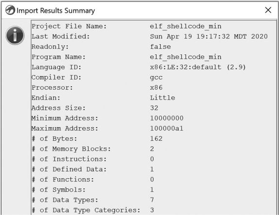
Figure 17-20: Import Results Summary window for the new ELF Shellcode Loader

If you open the file in the CodeBrowser and allow Ghidra to auto analyze the file, you should see the following ELF header definition at the top of the file:

10000000 7f             db      7Fh          e_ident_magic_num
10000001 45 4c 46       ds      "ELF"        e_ident_magic_str
10000004 01             db      1h           e_ident_class
10000005 01             db      1h           e_ident_data
10000006 01             db      1h           e_ident_version
10000007 00 00 00 00 00 db[9]                e_ident_pad
         00 00 00 00
10000010 02 00          dw      2h           e_type
10000012 03 00          dw      3h           e_machine
10000014 01 00 00 00    ddw     1h           e_version
10000018 54 00 00 10    ddw     shellcode➊  e_entry
1000001c 34 00 00 00    ddw     34h          e_phoff
10000020 00 00 00 00    ddw     0h           e_shoff
10000024 00 00 00 00    ddw     0h           e_flags
10000028 34 00          dw      34h          e_ehsize

Within the listing, the shellcode label ➊ is clearly associated with the entry point. Double-clicking the shellcode label takes you to a function, named shellcode, that contains the same shellcode contents we’ve seen in our previous two examples, including the following:

1000008c  JNS    LAB_10000086
1000008e  PUSH   "//sh"
10000093  PUSH   "/bin"
10000098  MOV    EBX,ESP
1000009a  PUSH   EAX

Now that you have confirmed that your new loader works, you can add it as an extension to your Ghidra installation and share it with your colleagues who have been anxiously awaiting this functionality.

Summary

In this chapter, we focused on the challenges associated with dealing with unrecognized binary files. We walked through examples of the loading and analysis processes that we can use within Ghidra to help us with these challenging reverse engineering scenarios. Finally, we extended our module creation capabilities to the world of Ghidra loaders.

While the examples that we built were trivial, they provided the foundation and introduced all of the components required to write more complex loader modules in Ghidra. In the next chapter, we round out our discussion of Ghidra modules with an introduction to processor modules—the components most responsible for the overall formatting of a disassembled binary.