
1
Introduction to Lasers
1.1 Introduction
Lasers are widely applied in academic, medical, industrial, and military research. They are also used beyond the boundary of research, in numerous engineering and manufacturing applications that continue to expand.
Optics principles and optical elements are applied to build laser resonators and to propagate laser radiation. Optical instruments are utilized to characterize laser emission and lasers have been incorporated into new optical instrumentation. This book focuses on the optics and optical principles needed to build lasers, the optical instrumentation necessary to characterize laser emission, and the laser-based optical instrumentation. The emphasis is on practical and utilitarian aspects of relevant optics including the necessary theory. Albeit this book refers explicitly to macroscopic lasers, many of the principles and ideas, described here, are applicable to microscopic lasers.
This book was written for advanced undergraduate physics students, non-optics graduate students using lasers, engineers, and scientists from other fields seeking to incorporate lasers and optics into their work.
This second edition is a revised, expanded, and improved version of its first edition (Duarte 2003). In addition to new and additional material on tunable lasers, this edition also includes some relevant topics of quantum optics as described in Quantum Optics for Engineers (Duarte 2014).
The organization of this book is fairly straightforward. It has three stages. It begins with an introduction to laser concepts and continues with Chapters 1 through 7 that introduce the ideas necessary to quantify the propagation of laser radiation and that are central to the design tunable laser oscillators. The second stage begins with Chapter 8 on nonlinear optics that has intra- and extracavity applications.
The attention is then focused on a survey of the emission characteristics of most well-known lasers with an added emphasis on tunable semiconductor and tunable solid-state lasers. The third stage includes Chapter 11 on interferometry that describes most well-known interferometers via Dirac’s quantum notation. This chapter is followed by Chapter 12 on the principles of spectrometry and dispersion-based instrumentation. In each chapter, a number of examples are described in detail to illustrate the applications of the theory. A set of fairly straightforward problems is added at the end of each chapter to assist the reader to assess the assimilation of the subject matter.
Thus, the book begins with an introduction to some basic concepts of laser excitation mechanisms and laser resonators in Chapter 1. The focus then turns to optical principles with Dirac optics being discussed in Chapter 2 and the uncertainty principle introduced in Chapter 3. The principles of dispersive optics are described in Chapter 4, whereas classical polarization is discussed in Chapter 5. Next, propagation matrices are introduced in Chapter 6. The optical principles discussed in Chapters 1 through 6 can all be applied to the design and construction of tunable laser oscillators as described in Chapter 7. Nonlinear optics, with an emphasis on frequency conversion, is outlined in Chapter 8. A brief but fairly comprehensive survey of gas lasers, liquid lasers, solid-state lasers, and semiconductor lasers is given in Chapter 9. The attention is focused on the emission characteristics of the various lasers. At this second stage, it is hoped that the student, or reader, should have gained sufficient confidence and familiarity with the subject of laser optics as to select an appropriate gain medium and resonator architecture for its efficient use in an applied field. The optical architecture and applications of N-slit laser interferometers are considered in Chapter 10, whereas interferometric based diagnostic instrumentation is described in Chapter 11. Dispersion-based spectrometry is described in Chapter 12. The book concludes with Chapter 13 with a survey of useful physical constants and optical quantities.
It should be emphasized that the material in this book does not require mathematical tools above those available to a third-year undergraduate physics student. Also, perhaps with the exception of Chapter 7, individual chapters can be studied independently. Finally, in this second edition, some equations and figures that are deemed important are reproduced again, when needed, rather than forcing the reader to go back to the text to find that material, thus easing the lecture process.
1.1.1 Historical Remarks
A considerable amount has been written about the history of the maser and the laser. For brief, and yet informative, historical summaries, the reader should refer to Willett (1974), Siegman (1986), Townes (1999), and Silfvast (2008). Here, remarks will be limited to mention that the first experimental visible laser was demonstrated by Maiman (1960), and this laser was an optically pumped solid-state laser. More specifically, it was a flashlamp-pumped ruby laser. This momentous development was followed shortly afterward by the introduction of the first electrically excited gas laser (Javan et al. 1961). This was the He–Ne laser emitting in the near infrared. From a practical perspective, the demonstration of these laser devices also signaled the birth of experimental laser optics since the laser resonators, or laser optical cavities, are an integral and essential part of the laser.
Two apparently unrelated publications on the laser are mentioned next. The first is the description that Dirac gave on interference in his book The Principles of Quantum Mechanics first published in 1930 (Dirac 1978). In his statement on interference, Dirac first refers to a source of monochromatic light, and then to a beam of light consisting of a large number of photons. In his discussion, it is this beam composed of a large number of undistinguishable photons that are divided and then recombined to undergo interference. In this regard, Dirac could have been describing a high-intensity laser beam with a very narrow linewidth (Duarte 1998). Regardless of the prophetic value of Dirac’s description, this was probably the first discussion, in physical optics, including a coherent beam of light. In other words, Dirac wrote the first chapter in Laser Optics (Duarte 2003).
The second publication of interest is The Feynman Lectures on Physics authored by Feynman et al. (1965). In Chapter 9 of the volume on quantum mechanics, Feynman uses Dirac’s notation to describe the quantum mechanics of stimulated emission. In Chapter 10, he applies that physics to several physical systems, including dye molecules. Notice that this was done just prior to the discovery of the dye laser by Sorokin and Lankard (1966) and Schäfer et al. (1966). In this regard, Feynman could have predicted the existence of the tunable laser (Duarte 2003). Further, he made accessible Dirac’s quantum notation via his thought experiments on two-slit interference with electrons. This provided the foundations for the subject of Dirac optics described in Chapter 2 where the method outlined by Feynman is extended to generalized transmission gratings using photons rather than electrons.
1.2 Lasers
The word laser has its origin in an acronym of the words light amplification by stimulated emission of radiation. Although the laser is readily associated with the spatial and spectral coherence characteristics of its emission, to some the physical meaning of the concept still remains shrouded in mystery. Looking up the word laser in a good dictionary does not help much.
A laser is a device that transforms electrical energy, chemical energy, or incoherent optical energy, into coherent optical emission. This coherence is both spatial and spectral. Spatial coherence means a highly directional light beam, with little divergence, whereas spectral coherence means an extremely pure color of emission. An alternative way to cast this idea is to think of the laser as a device that transforms ordinary energy into an extremely well-defined form of energy in both the spatial and the spectral domain. However, this is only the manifestation of the phenomenon since the essence of this energy transformation lies in the device called laser.
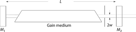
FIGURE 1.1 Basic laser resonator. It is composed of an atomic, or molecular, gain medium and two mirrors aligned along the optical axis. The length of the cavity is L, and the diameter of the beam is 2w. The gain medium can be excited optically or electrically.
Physically, the laser consists of an atomic or molecular gain medium optically aligned within an optical resonator or optical cavity as depicted in Figure 1.1. When excited by electrical energy, or optical energy, the atoms or molecules in the gain medium oscillate at optical frequencies. This oscillation is maintained and sustained by the optical resonator or optical cavity. In this regard, the laser is analogous to a mechanical or radio oscillator but oscillates at extremely high frequencies. For the green color of λ = 500 nm, the equivalent frequency is ν ≈ 5.99 × 10¹⁴. Hz. A direct comparison between a laser and a radio oscillator makes the atomic or molecular gain medium equivalent to the transistor and the elements of the optical cavity equivalent to the resistances, capacitances, and inductances. Thus, from a physical perspective, the gain medium in conjunction with the optical cavity behaves like an optical oscillator (Duarte 1990a). The spectral purity of the emission of a laser is related to how narrow its linewidth is. High-power narrow-linewidth lasers can have linewidths of ΔQ ≈ 300 MHz, low-power narrow-linewidth lasers can have ΔQ ≈ 100 kHz, while stabilized lasers can yield ΔQ ≈ 1 kHz, or even much narrower linewidths. In all the instances mentioned here, the emission is in the form of a single longitudinal mode, that is, all the emission radiation is contained in a single electromagnetic mode.
In the language of the laser literature, a laser emitting narrow-linewidth radiation is referred to as a laser oscillator or a master oscillator (MO). High-power narrow-linewidth emission is attained when a MO is used to inject a laser amplifier or a power amplifier (PA). Large high-power systems include several MOPA chains, with each chain including several amplifiers. The difference between an oscillator and an amplifier is that the amplifier simply stores energy to be released up on the arrival of the narrow-linewidth oscillator signal. In some cases, the amplifiers are configured within unstable resonator cavities in what is referred to as a forced oscillator (FO). When that is the case, the amplifier is called a FO and the integrated configuration is referred to as a MOFO system. This subject is considered in more detail in Chapter 7.
1.2.1 Laser Optics
Laser optics refers to the individual optics elements that comprise laser cavities, the optics ensembles that comprise laser cavities, and the physics that results from the propagation of laser radiation. In addition, the subject of laser optics includes instrumentation employed to characterize laser radiation and instrumentation that incorporates lasers.
One of the main functions, and perhaps the principal function, of skillfully designed properly applied laser optics is to produce high-quality coherent emission for utilitarian purposes. The essence of high-quality coherent radiation is single-transverse-mode (TEM00), and narrow-linewidth single-longitudinal-mode (SLM), emission.
1.2.2 Laser Categories
Lasers emitting radiation confined in TEM00 beams, and characterized as narrow-linewidth emission sources, are used in a variety of applications in research and development laboratories. These lasers can be categorized in two classes:
Narrow-linewidth tunable lasers, used in applications such as communications, laser cooling, laser isotope separation, medicine, metrology, and spectroscopy
Narrow-linewidth fixed-frequency lasers, used in applications such as imaging, medicine, metrology, and material processing
Lasers emitting radiation confined in TEM00 beams, and characterized as ultra-short-pulse emission, are mainly used in spectroscopy and the study of light-matter interactions.
1.3 Excitation Mechanisms and Rate Equations
There are various methods and approaches to describe the dynamics of excitation in the gain media of lasers. Approaches range from complete quantum mechanical treatments to rate equation descriptions (Haken 1970). A complete survey of energy-level diagrams corresponding to gain media in the gaseous, liquid, and solid states is given by Silfvast (2008). Here, a basic description of laser excitation mechanisms is given using energy levels and classical rate equations applicable to tunable molecular gain media. The link to the quantum mechanical nature of the laser is made via the cross sections of the transitions.
1.3.1 Rate Equations
Rate equations are widely applied in physics and laser physics in particular. They, for example, can be used to describe and quantify the process of molecular recombination in metal vapor lasers or to describe the dynamics of the excitation mechanism in a multiple-level gain medium. Here, the basic concept of rate equations is introduced using dye laser gain media as a vehicle, but the principles also apply to gas and solid-state gain media. Organic laser dyes are rather large molecules with molecular weights ranging from ~175 to ~830 mu. Dye lasers using this class of gain media have been shown to span with their emission the electromagnetic spectrum from the near ultraviolet to the near infrared. Figure 1.2 illustrates the wavelength coverage provided by three classes of dye molecular species: the coumarins, the xanthenes, and the cyanines. Figure 1.3 depicts the dye molecular structure of the laser dye coumarin 545 tetramethyl (C545T), which has a molecular weight of 430.56 mu. In a polarization-selective mirror-grating cavity, C545T provides a fairly large laser intensity dynamic range and an excellent tunability in the 501 ≤ λ ≤ 574 nm range as shown in Figure 1.4 (Duarte et al. 2006).
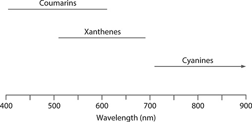
FIGURE 1.2 Approximate emission ranges for three classes of laser dyes: the coumarins, the xanthenes, and the cyanines. The rhodamines belong to the xanthenes. The cyanines reach up to 1100 nm. The wavelength range shown is covered using several laser dyes.
An ideally simplified two-level molecular system is depicted in Figure 1.5. Here, the pump excitation intensity Ip(t) populates the upper energy level N1 from the ground state N0. Emission from the upper state is designated as Il(x, t, λ) since it is a function of position x in the gain medium, time t, and wavelength λ. The time evolution of the upper- or excited-state population can be written as
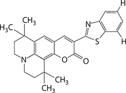
FIGURE 1.3 Molecular structure of C545T. This laser dye has a molecular weight of 430.56 mu. (Reproduced with permission from Duarte, F.J., et al., J. Opt. A: Pure Appl. Opt., 8: 172–174. Copyright 2006, Institute of Physics.)

FIGURE 1.4 Wavelength tuning range of a grating mirror laser cavity using C545T as gain medium. (Reproduced with permission from Duarte, F.J., et al., J. Opt. A: Pure Appl. Opt. 8: 172–174. Copyright 2006, Institute of Physics.)

FIGURE 1.5 Simple two-level energy system including a ground level and an upper level.
∂N1∂t=N0σ0,1Ip(t)-N1σeIl(x,t,λ)(1.1)
which has a positive term due to excitation from the ground level and a negative component due to the emission from the upper state. Here, σ01, is the absorption cross section and σe is the emission cross section. Cross sections have units of cm2, time has units of seconds (s), the populations have units of molecules cm−3, and the intensities have units of photons cm−2 s−1.
The pump intensity Ip (t) undergoes absorption due to its interaction with a molecular population N0. A process that is described by the equation
c-1[∂Ip(t)∂t]=-N0σ0,1Ip(t)(1.2)
where:
c is the speed of light
The process of emission is described by the time evolution of the intensity Il (x, t, λ) given by
c-1[∂Il(x,t,λ)∂t]+[∂Il(x,t,λ)∂x]=(N1σe-N0σl0,1)Il(x,t,λ)(1.3)
In the steady state, this equation reduces to
[∂Il(x,λ)∂x]≈(N1σe-N0σl0,1)Il(x,λ)(1.4)
which can be integrated to yield
![]()
Thus, if N1σe>N0σl0,1
1.3.2 Dynamics of Multiple-Level System
In this section, the rate equation approach is used to describe in some detail the excitation dynamics in a multiple-level energy system relevant to a well-known tunable molecular laser known as the dye laser. This approach applies to laser dye gain media in either the liquid or the solid state. The literature on rate equations for dye lasers is fairly extensive, which includes the works of Ganiel et al. (1975), Teschke et al. (1976), Penzkofer and Falkenstein (1978), Dujardin and Flamant (1978), Munz and Haag (1980), Haag et al. (1983), Nair and Dasgupta (1985), Hillman (1990), Schäfer (1990), and Jensen (1991). An energy-level diagram for a laser dye molecule is depicted in Figure 1.6.

FIGURE 1.6 Energy-level diagram corresponding to a laser dye molecule, which includes three electronic levels (S0, S1, and S2) and two triplet levels (T1 and T2). Each electronic level contains a large number of vibrational and rotational levels. Laser emission takes place due to S1 → S0 transitions.
Usually, three electronic states S0, S1, and S2 are considered in addition to two triplet states T1 and T2, which are detrimental to laser emission. Laser emission takes place due to S1 → S0 transitions. Each electronic state contains a large number of overlapping vibrational–rotational levels. This plethora of closely lying vibrational– rotational levels is what gives origin to the broadband gain and the intrinsic tunability of dye lasers. This is because E = hν, where ν is frequency. Thus, a change in energy ΔE implies a change in frequency Δν, which also means a change in the wavelength domain or Δλ.
In reference to the energy-level diagram of Figure 1.6, and considering only vibrational manifolds at each electronic state, a set of rate equations for transverse excitations was written by Duarte (1995a):
N=m∑S=0m∑v=0NS,v+m∑T=1m∑v=0NT,v(1.6)
∂N1,0∂t≈∑mv=0N0,vσ0,10,vIp(t)+∑mv=0N0,vσl0,10,vIl(x,t,λv)+N2,0τ2,1-N1,0[∑mv=0σ1,20,vIp(t)+∑mv=0σe0v,Il(x,t,λv)+∑mv=0σl1,20,vIl(x,t,λv)+(kS,T+τ-11,0)](1.7)
∂NT1,0∂t≈N1,0kS,T-NT1,0τT,S-NT1,0[m∑v=0σT1,20,vIP(t)+m∑v=0σTl1,20,vIl(x,t,λv)](1.8)
c-1∂IP(t)∂t≈-(N0,0m∑v=0σ0,10,v+N1,0m∑v=0σ1,20,v+NT1,0m∑v=0σT1,20,v)IP(t)(1.9)
c-1∂Il(x,t,λ)∂t+∂Il(x,t,λ)∂x≈N1,0∑mv=0σe0,vIl(x,t,λv)-∑mv=0N0,vσl0,10,vIl(x,t,λv)-N1,0∑mv=0σl1,20,vIl(x,t,λv)-NT1,0∑mv=0σTl1,20,vIl(x,t,λv)(1.10)
Il(x,t,λ)=m∑v=0Il(x,t,λv)(1.11)
Il(x,t,λ)=I+l(x,t,λ)+I-l(x,t,λ)(1.12)
In this set of equations, frequency dependence is incorporated via the summation terms and variables depending on the vibrational assignment v. Now, using the style of Duarte (2014), the equation parameters are as follows (see Figure 1.6):
Ip(t) is the intensity of the pump laser beam. Units are photons cm−2 s−1.
Il(x,t,λ) is the laser emission from the gain medium. Units are photons cm−2 s−1.
NS,v refers to the population of the S electronic state at the v vibrational level. It is given as a number per unit volume (cm−3).
NT,v refers to the population of the T triplet state at the v vibrational level. It is given as a number per unit volume (cm−3).
The absorption cross sections, such as σ0,10,v
σ0,10,v , are identified by a subscript S″, S′v″,v′ that refers the electronic S″ → S′ transition and the vibrational transition v″ → v′. The same convention applies to the triplet levels. Units are cm2.The emission cross sections, σe0,v
σe0,v , are identified by the subscript e′v′,v″ Vibrational transitions denoting emission are designated v′ → v″. Units are cm2.Radiationless decay times, such as W10,, are identified by subscripts that denote the corresponding S′ → S″ transition. Units are s.
kS,T, is a radiationless decay rate from the singlet to the triplet. Units are s−1.
The broadband nature of the emission is a consequence of the involvement of the vibrational manifold of the ground electronic state represented by the summation terms of Equations 1.9 through 1.11. The usual approach to solve an equation system as described here is numerical.
Since the gain medium exhibits homogeneous broadening, the introduction of intracavity frequency selective optics (see Chapter 7) enables all the molecules to contribute efficiently to narrow-linewidth emission.
A simplified set of equations can be obtained by replacing the vibrational manifolds by single energy levels and by neglecting a number of mechanisms including spontaneous decay from S2 and absorption of the pump laser by T1. Thus, Equations 1.6 through 1.10 reduce to
N=N0+N1+NT(1.13)
∂N1∂t≈N0σ0,1Ip(t)+(N0σl0,1-N1σe-N1σl1,2)Il(x,t,λ)-N1(kS,T+τ-11,0)(1.14)
∂NT∂t=N1kS,T-NTτ-1T,S-NTσTl1,2Il(x,t,λ)(1.15)
c-1∂Ip(t)∂t=-(N0σ0,1+N1σ1,2)Ip(t)(1.16)
c-1[∂Il(x,t,λ)∂t]+[∂Il(x,t,λ)∂x]=(N1σe-N0σl0,1-N1σl1,2-NTσTl1,2)Il(x,t,λ)(1.17)
This set of equations is similar to the set of equations considered by Teschke et al. (1976). This type of equations has been applied to simulate numerically the behavior of the output intensity and the gain as a function of the laser–pump intensity and to optimize laser performance. Relevant cross sections and excitation rates are given in Tables 1.1 and 1.2.
For long-pulse, or continuous-wave (CW) excitation, the time derivatives approach zero and Equations 1.14 through 1.17 reduce to
N0σ0,1Ip+(N0σl0,1-N1σe-N1σl1,2)Il(x,λ)=N1(kS,T+τ-11,0)(1.18)
N1kS,T=NTτ-1T,S+NTσTl1,2Il(x,λ)(1.19)
N0σ0,1=-N1σ1,2(1.20)
TABLE 1.1
Molecular Transition Cross Sections for Rhodamine 6G
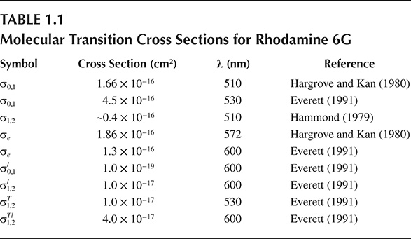
TABLE 1.2
Molecular Transition Rates and Decay Times for Rhodamine 6G
Symbol |
Rate (s−1) |
Time (s) |
Reference |
kS,T |
2.0 × 10⁷ |
Everett (1991) |
|
τT ,S |
0.5 × 10⁻⁷ |
Everett (1991) |
|
τ1,0 |
3.5 × 10⁻⁹ |
Everett (1991) |
|
τ2,1 |
~1.0 × 10⁻¹² |
Hargrove and Kan (1980) |
∂Il(x,λ)∂x=(N1σe-N0σl0,1-N1σl1,2-NTσTl1,2)Il(x,λ)(1.21)
From these equations, some characteristic features of CW dye lasers become apparent.
1.3.2.1 Example
As indicated by Dienes and Yankelevich (1998), from Equation 1.18 just below threshold, that is, Il (x,λ) ≈ 0,
Ip≈σ-10,1(kS,T+τ-110)N1N0(1.22)
which means that to approach population inversion, using rhodamine 6G under visible laser excitation, pump intensities exceeding 1022 photons cm−2 s−1 are necessary.
1.3.2.2 Example
A problem unique to long-pulse and CW dye lasers is intersystem crossing from N1 into T1. Thus, researchers use triplet-level quenchers such as O2 and C8H8 (see, e.g., Duarte 1990) to neutralize the effect of that level. Under these circumstances, from Equation 1.21, the gain factor can be written as
g=[N1(σe-σl1,2)-N0σl0,1]L(1.23)
From this equation, it can be deduced that amplification can occur in the absence of triplet losses, when the ratio of the populations becomes
N1N0>σl0,1σe-σl1,2(1.24)
From the values of the cross sections available in Table 1.1, this ratio can be approximately (10-19/10-16) ≈ 0.001.
1.3.3 Transition Probabilities and Cross Sections
The dynamics described with the classical approach of rate equations depends on the cross sections listed in Table 1.1, which are measured experimentally. The origin of these cross sections, however, is not classical. Its origin is quantum mechanical. Here, the quantum mechanical probability for a two-level transition is introduced and its relation to the cross section of the transition is outlined. The style adopted here follows the treatment given to this problem by Feynman et al. (1965) which uses Dirac notation. An introduction to Dirac notation is given in Chapter 2.
This approach is based on the basic Dirac principles of quantum mechanics described by
〈ϕ|ψ〉=∑j〈ϕ|j〉〈j|ψ〉(1.25)
and
〈ϕ|ψ〉=〈ψ|ϕ〉*(1.26)
For j = 1, 2, Equation 1.25 leads to
〈(ϕ|ψ〉=〈ϕ|2〉〈2|ψ〉+〈ϕ|1〉〈1|ψ〉(1.27)
which can be expressed as
〈ϕ|ψ〉=〈ϕ|2〉C2+〈ϕ|1〉C1(1.28)
where:
C1=〈1|ψ〉(1.29)
and
C2=〈2|ψ〉(1.30)
Here, the amplitudes change as a function of time according to the Hamiltonian
ihdCjdt=2∑kHjkCk(1.31)
Now, Feynman et al. (1965) define new amplitudes CI and CII as linear combinations of C1 and C2. However, since
〈II|II〉=〈II|1〉〈1|II〉+〈II|2〉〈2|II〉(1.32)
must equal unity, the normalization factor 2−1/2 is introduced in the definitions of the new amplitudes
CII=1√2(C1+C2)(1.33)
and
CI=1√2(C1-C2)(1.34)
For a molecule under the influence of an electric field, the components of the Hamiltonian are
H11=E0+μℇ(1.35)
H12=-A(1.36)
H21=-A(1.37)
H22=E0-μℇ(1.38)
where
ℇ=ℇ0(eiωt+e-iωt)(1.39)
μ corresponds to the electric dipole moment
Expanding the Hamiltonian given in Equation 1.31, and then subtracting and adding yield
iħdCIdt=(E0+A)CI+μℇCII(1.40)
iħdCIIdt=(E0-A)CII+μECI(1.41)
Assuming a small electric field, the solutions are of the form:
CI=DIe-iEII/ℏt(1.42)
CII=DIIe-iEII/ℏt(1.43)
where:
EI=E0+A(1.44)
and
EII=E0-A(1.45)
Hence, neglecting the term (ω + ω0) because it oscillates too rapidly to contribute to the average value of the rate of change of DI and DII, the following expressions DI and DII are found:
iħdDIdt=μℇ0DIIe-i(ω-ω0)t(1.46)
iħdDIIdt=μℇ0DIei(ω-ω)t0(1.47)
If at t = 0, DI ≈ 1, then integration of Equation 1.46 yields (Feynman et al. 1965)
DII=μℇ0ħ[1-ei(ω-ω0)Tω-ω0](1.48)
and following multiplication with its complex conjugate
|DII|2=(μℇ0ħ)2[2-2cos(ω-ω0)T(ω-ω0)2](1.49)
which can be written as (Feynman et al. 1965)
|DII|2=(μℇ0Tħ)2sin2[12(ω-ω0)T][12(ω-ω0)T]2(1.50)
which is the probability of the transition I → II. It can be further shown that
|DI|2Tab=|DII|2(1.51)
which means that the probability of emission is equal to the probability of absorption. This result is central to the theory of absorption and radiation of light by atoms and molecules.
Using ⁈=2ε0cℇ20, and replacing μ by 3−1/2μ (Sargent et al. 1974), the expression for the probability of the transition becomes
|DII|2=2π3(μ2T24πε0cħ2ℐ(ω0)sin2[12(ω-ω0)T][12(ω-ω0)T]2(1.52)
where:
μ is the dipole moment in units of Cm
(1/4πɛ0) is in units of Nm2 C−2
ℐ (ω0) is the intensity in units of J s−1 m−2
Integrating Equation 1.52 with respect to the frequency ω, the dimensionless transition probability becomes
|DII|2=4π23(μ24πε0cħ2)[ℐ(ω0)Δω]T(1.53)
It then follows that the cross section for the transition can be written as
σ=4π23(μ24πε0cħI(ωΔω)(1.54)
in units of m2 (although the more widely used unit is cm2; see Table 1.1). For a simple atomic or molecular system, the dipole moment can be calculated from the definition (Feynman et al. 1965)
μmnξ=〈m|H|n〉=Hmn(1.55)
where:
Hmnis the matrix element of the Hamiltonian
For diatomic molecules, the dependence of this matrix element on the Franck– Condon factor (qv′,v″) and the square of the transition moment (|R|2e) is described by Chutjian and James (1969). Byer et al. (1972) wrote an expression for the gain of vibrational–rotational transitions of the form
g=σNL(1.56)
or more specifically
g=4π23(14πε0cℏ)(ωΔω)|Re|2qv′,v′′[SJ′′(2J′′+1)]NL(1.57)
where:
SJ″ is known as the line strength
J″ identifies a specific rotational level
In practice, however, cross sections are mostly determined experimentally as in the case of those listed in Table 1.1.
Going back to Equation 1.53, and rearranging its terms, it follows that the intensity can be expressed as a function of the transition probability (Duarte 2014)
ℐ(ω0)=3π(ε0ch2μ2)(ΔωT)|DII|2(1.58)
or
ℐ(ω0)=3πκ(ΔωT)|DII|2(1.59)
with
κ=(ε0cħ2μ2I(1.60)
where the units for the constant N are J s m−2. Subsequently, the intensity ℐ (ω0) has units of J s−1 m−2 or W m−2.
1.3.3.1 Example
Within resonance, where Δω ≈ 2π/T, Equation 1.53 can be approximated as
|DII|2≈π3(μ2ε0cħ2)2π(Δω)2ℐ(ω0)(1.61)
which can be reexpressed as
ℐ(ω0)≈32π2κ(Δω)2|DII|2(1.62)
This approximation indicates that the intensity is proportional to the square of the frequency difference multiplied by the probability of the transition, or (Δω)2|DII|2, and is given in units of J s−1 m−2 or W m−2.
1.4 The Schrödinger Equation and Semiconductor Lasers
The Schrödinger equation is central to the emission properties of semiconductor lasers that are widely tunable sources of coherent radiation in various important segments of the electromagnetic spectrum, as illustrated in Figure 1.7.
The Schrödinger equation can be derived via Schrödinger’s way (Schrödinger 1926), a heuristic path, or Dirac’s notation. Here, the Schrödinger equation is introduced via a heuristic path originally sketched by Haken (1981) and via Dirac’s notation in an approach modeled after Feynman et al. (1965), as recently reviewed by Duarte (2014).
1.4.1 A Heuristic Introduction to the Schrödinger Equation
This approach uses a mixture of classical, relativistic, and quantum concepts. The presentation given here follows the review given by Duarte (2014), which was modeled using concepts outlined by Haken (1981). This heuristic approach begins by considering a free particle moving with classical kinetic energy

FIGURE 1.7 Approximate wavelength range covered by various types of semiconductors used in tunable lasers. This is only an approximate depiction and some of the ranges might not be continuous. Not shown are the InGaAs/InP semiconductors that emit between 1600 and 2100 nm or the quantum cascade lasers that emit deep into the infrared (see Chapter 9).
E=12mv2(1.63)
and using p = mv, the kinetic energy equation can be restated as
E=p22m(1.64)
Next, using Planck’s quantum energy (Planck 1901),
E=hv
in conjunction with λ = c/ν, and E = mc2, the de Broglie expression for momentum can be expressed as (de Broglie 1923)
p=ħk(1.65)
The next step consists in incorporating the classical “wave functions of ordinary wave optics” (Dirac 1978)
ψ(x,t)=ψ0e-i(ωt-kx)(1.66)
whose derivative with respect to time becomes
∂ψ(x,t)∂t=(-iω)ψ0e-i(ωt-kx)(1.67)
Similarly, the first and second derivatives with respect to displacement are
∂ψ(x,t)∂x=(+ik)ψ0e-i(ωt-kx)(1.68)
and
∂2ψ(x,t)∂x2=(-k2)ψ0e-i(ωt-kr)(1.69)
Multiplying the first time derivative by (−iħ) yields
-iħ∂ψ(x,t)∂t=(-ħω)ψ0e-i(ωt-kx)(1.70)
and multiplying the second displacement derivative by (−ħ2/2m) yields
ħ22m∂2ψ(x,t)∂x2=ħ2k22mψ0e-i(ωt-kx)(1.71)
Recognizing that E = ħ2k2/2m,
ħ22m∂2ψ(x,t)∂x2=+iħ∂ψ(x,t)∂t(1.72)
which is the basic form of Schrödinger’s equation. As can be seen, this heuristic approach to Schrödinger’s equation utilizes Planck’s quantum energy, the classical kinetic energy of a free particle, and the classical “wave functions of ordinary wave optics.” That is, Schrödinger’s equation describes the motion of a free particle propagating in according to ordinary wave optics. The crucial quantum step consists in incorporating, in the development, Planck’s energy equation E = hν. Once again, the central role of classical wave equation equations of the form
ψ(x,t)=ψ0e-i(ωt-kr)
is highlighted.
1.4.2 The Schrödinger Equation Via dirac’s Notation
As explained in Section 1.4.1, the Hamiltonian Hij is related to the time-dependent amplitude Ci by (Dirac 1978)
iħdCidt=∑jHijCi(1.73)
For C〈i|ψ〉, this equation can be rewritten as
iħd〈i|ψ〉dt=∑j〈i|H|j〉〈j|ψ〉(1.74)
which, for i = x, can be written as
iħd〈x|ψ〉dt=∑j〈x|H|x′〉〈x′|ψ〉(1.75)
Since 〈x|ψ〉 = ψ(x), this equation can be reexpressed as
iħdψ(x)dt=∫H(x,x′)ψ(x′)dx′(1.76)
The integral on the right-hand side is given by
∫H(x,x′)ψ(x′)dx′=-ħ22md2ψ(x)dx2+V(x)ψ(x)(1.77)
According to Feynman, the right-hand side of the above equation simply came “from the mind of Schrödinger” (Feynman et al. 1965). A methodical description of the Schrödinger approach is given by Duarte (2014).
Next, combining Equations 1.76 and 1.77, we get the formal Schrödinger equation
+iħdψ(x)dt=-ħ22md2ψ(x)dx2+V(x)ψ(x)(1.78)
In three dimensions, the wave function becomes ψ(x,y,z), the potential is V(x,y,z), and introducing
∇2=∂22+∂22+∂22(1.79)
and Schrödinger’s equation in three dimensions takes the succinct form
+iħ∂ψ∂t=-ħ22m∇2ψ+Vψ(1.80)
1.4.3 The Time-Independent Schrödinger Equation
As suggested by Feynman, using a solution of the form
ψ(x)=Ψ(x)e-iEt/ℏ(1.81)
Equation 1.80, in one dimension, becomes
∂2Ψ(x)∂x2-2mħ2[V(x)-E]Ψ(x)=0(1.82)
or
∂2Ψ(x)∂x2=2mħ2[V(x)-E]Ψ(x)(1.83)
which is known as the one-dimensional time-independent Schrödinger equation. This simple form of the Schrödinger equation is of enormous significance to semiconductor physics and semiconductor lasers.
1.4.4 Semiconductor Emission
The description of semiconductor photon emission can be described using the time-independent Schrödinger equation
∂2Ψ(x)∂x2-2mħ2[V(x)-E]Ψ(x)=0(1.84)
and using the spatial component of the wave function as solution
Ψ(x)=Ψ0e-ikx(1.85)
leads directly to
E=k2ħ22m+V(x)(1.86)
This energy expression is the sum of kinetic and potential energy (E = EK + EP) so that
EK+EP=k2ħ22m+V(x)(1.87)
and
EK=k2ħ22m(1.88)
The kinetic energy EK as a function of the wave number k = 2π/λ is shown graphically in Figure 1.8. The graph is a positive parabola for positive values of m and is known as the conduction band. The negative parabola is known as the valence band. The separation between the two bands is known as the band gap, EG. If an electron is excited and a transition from the valence band to the conduction band occurs, it is said to leave behind a vacancy or hole. Under certain conditions, radiation might also occur higher from the conduction band as suggested in Figure 1.9; however, such process is undermined by fast phonon relaxation.
1.4.4.1 Example
Electrons can transition from the bottom of the conduction band to the top of valence band by recombining with holes. For a material such as gallium arsenide (GaAs), the band gap at T = 300°K is EG ≈ 1.43 eV (Kittel 1971). Now, using the conversion 1eV 1.602176565 × 10⁻¹⁹ J, h = 6.62606957 × 10⁻³⁴ Js, c = 2.99792458 × 10⁸ ms-1 (see Chapter 13), and Planck’s energy equation E = hν,
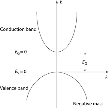
FIGURE 1.8 Conduction and valence bands according to EK = ±(k2ħ2/2m) (Reproduced from Duarte, F.J., Quantum Optics for Engineers, CRC Press, New York, 2014. With permission from Taylor & Francis.)
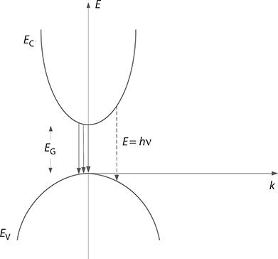
FIGURE 1.9 Emission due to recombination transitions from the bottom of the conduction band to the top of the valence band. (Reproduced from Duarte, F.J., Quantum Optics for Engineers, CRC Press, New York, 2014. With permission from Taylor & Francis.)
λ=chE≈867.02 nm
In other words, the recombination emission occurs around 867 nm. Here, it should be noted that the energy band gap varies as a function of temperature so that at T = 0°K it is EG ≈ 1.52 eV (Kittel 1971), which would change the wavelength to λ ≈ 815.68 nm, thus demonstrating one avenue to tune the wavelength.
1.4.5 Quantum Wells
Starting with a potential well as described by Silfvast (2008), V(x) = 0 for 0 <x < L and V(x) = ∞ for x = 0 or x = L, illustrated in Figure 1.10, then Equation 1.84
∂2Ψ(x)∂x2-2mħ2[V(x)-E]Ψ(x)=0
becomes
∂2Ψ(x)∂x2+2mħ2EΨ(x)=0(1.89)
for 0 < x < L. This is a wave equation of the form
d2Ψ(x)dx2+k2xΨ(x)=0(1.90)
where:
k2x=2mch2E(1.91)
The solution to Equation 1.90 is
Ψ(x)=sinkxx(1.92)
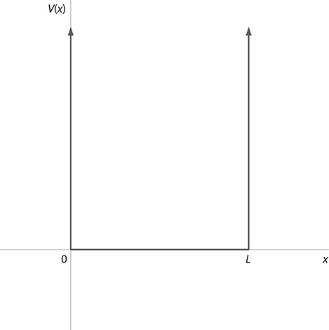
FIGURE 1.10 Potential well V(x) = 0 for 0 < x < L and V(x) = ∞ for x = 0 or x = L. (Reproduced from Duarte, F.J., Quantum Optics for Engineers, CRC Press, New York, 2014. With permission from Taylor & Francis.)
Since ψ(x) = 0 at x = 0 or x = L, we have
kx=nπL(1.93)
for n = 1, 2, 3,.... Substituting Equation 1.93 into 1.91 leads to
E=n2π2ħ22mcL2(1.94)
which should be labeled as En to account for the quantized nature of the energy, that is,
En=n2π2ħ22mcL2(1.95)
This quantized energy En indicates a series of possible discrete energy levels above the lowest point of the conduction band so that the total energy above the valence band becomes (Silfvast 2008)
E=Ec+En(1.96)
1.4.6 Quantum Cascade Lasers
Quantum cascade lasers (QCL; Faist et al. 1994) are tunable sources emitting in the infrared from a few micrometers to beyond 20 μm (see Chapters 7 and 9). These lasers operate via transitions between quantized levels within the conduction band of multiple-quantum well structures. The carriers involved are electrons generated in an n-doped material. A single stage includes an injector and an active region. The electron is injected into the active region at n2 and the transition occurs down to n1 (see Figure 1.11). Following emission, the electron continues into the next injector region. Practical devices include a series of such stages. From Equation 1.94, the energy difference between the two levels can be expressed as
ΔE=(n22-n21)π2ħ22mcL2(1.97)
where:
L is the thickness of the well
For n2 = 3 and n1 = 2, Equation 1.97 becomes (Silfvast 2008)
ΔE=(32-22)π2ħ22mcL2(1.98)
which is applicable to the 3 → 2 transition in GaInAs reported by Faist et al. (1994). As a footnote, it should be mentioned that the quantum well approach illustrated here also applies, with some modifications to the description of quantum wells in laser dye molecules (Schäfer 1990).
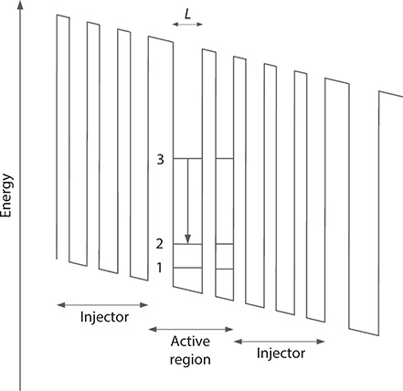
FIGURE 1.11 Simplified illustration of a multiple-quantum well structure relevant to quantum cascade lasers. An electron is injected from the injector region into the active region at n2 3. Thus, a photon is emitted via the 3 → 2 transition. The electron continues to the next region where the process is repeated. By configuring a series of such stages, one electron can generate the emission of numerous photons. (Reproduced from Duarte, F.J., Quantum Optics for Engineers, CRC Press, New York, 2014. With permission from Taylor & Francis.)
1.4.6.1 Example
Using ΔE = hν, in Equation 1.97, it follows that the wavelength of emission is given by
λ=(n22-n21)-18mccL2h(1.99)
This expression can be used to provide an estimate of the emission wavelength for a QCL transition, provided the effective mass, relevant to the emitting semiconductor, and the thickness of the quantum well (L) are known (see Problem 1.6).
1.4.7 Quantum Dots
Besides the multiple-quantum well configurations, other interesting semiconductor geometries include the quantum wire and the quantum dot. The quantum wire narrowly confines the electrons and holes in two directions (x,y). The quantum dot geometry severely confines the electrons in three dimensions (x,y,z). Under these circumstances, the quantized energy can be expressed as
E=Ec+k2xħ22mc+k2yħ22mc+k2xħ22mc(1.100)
where:
kx, ky, kz are defined according to Equation 1.93
The concept of quantum dot is not limited to semiconductor materials, but it also applies to nanoparticle gain media and nanoparticle core–shell gain media. For instance, for core–shell nanoparticles, the physics can be described with a Schrödinger equation of the form
∇2Ψ(r)-2mħ2[V(r)-E]Ψ(r)=0(1.101)
with the potential V(r) defined by the core–shell geometry (Dong et al. 2013).
1.5 Introduction to Laser Resonators and Laser Cavities
A basic laser is composed of a gain medium, a mechanism to excite that medium, and an optical resonator and/or optical cavity. These optical resonators and optical cavities, known as laser resonators and laser cavities, are the optical systems that reflect radiation back to the gain medium and determine the amount of radiation to be emitted by the laser. In this section, a brief introduction to laser resonators is provided. In further chapters, Chapter 7 in particular, this subject is considered in more detail.
The most basic resonator, regardless of the method of excitation, is that composed of two mirrors aligned along a single optical axis as depicted in Figure 1.1. In this flat-mirror resonator, one of the mirrors iŝ100% reflective, at the wavelength or wavelengths of interest, and the other mirror is partially reflective. The amount of reflectivity depends on the characteristics of the gain medium. The optimum reflectivity for the output coupler is often determined empirically. For a low-gain laser medium, this reflectivity can approach 99%, whereas for a high-gain laser medium, the reflectivity can be as low as 20%. In Figure 1.1, the gain medium is depicted with its output windows at an angle relative to the optical axis. If the angle of incidence of the laser emission on the windows is the Brewster angle, then the emission will be highly linearly polarized. If the windows are oriented as depicted in Figure 1.1, then the laser emission will be polarized parallel to the plane of incidence. An alternative to the flat-mirror approach is to use a pair of optically matched concave mirrors. Transverse and longitudinal excitation geometries are depicted in Figure 1.12. Further, in some resonators, the back mirror can be replaced by a diffraction grating as shown in Figure 1.13. This is often the case in tunable lasers.
These resonators might incorporate intracavity frequency-selective optical elements, such as Frabry–Perot etalons (Figure 1.13b), to narrow the emission line-width. They can also include intracavity beam expanders to protect optics from optical damage and to be utilized in linewidth narrowing techniques as described in Chapter 4. Resonators that yield highly coherent or narrow-linewidth emission are often called oscillators and are considered in detail in Chapter 7.
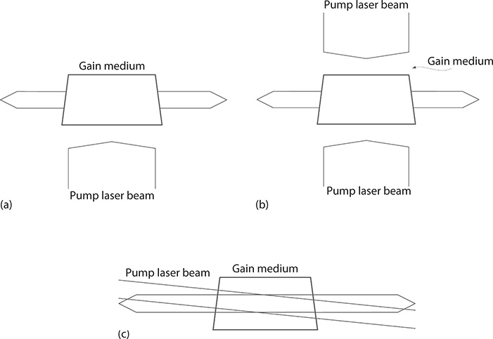
FIGURE 1.12 (a) Transverse laser excitation. (b) Transverse double-laser excitation. (c) Longitudinal laser excitation.
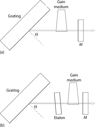
FIGURE 1.13 (a) Grating mirror resonator and (b) grating mirror resonator incorporating an intracavity etalon.
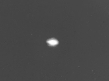
FIGURE 1.14 Cross section of a TEM00 laser beam from a high-power narrow-linewidth dispersive laser oscillator. The spatial intensity profile of this beam is near-Gaussian. (Reprinted from Opt. Commun., 117, Duarte, F.J., Solid-sate dispersive dye laser oscillator: Very compact cavity, 480–484, Copyright 1995b, with permission from Elsevier.)
The transverse mode structure in these resonators is approximately determined by the ratio (Siegman 1986)
NF=w2Lλ(1.102)
known as the Fresnel number. Here, w is the beam waist at the gain region, L is the length of the cavity, and λ is the wavelength of emission. The lower this number, the better the beam quality of the emission, or the closer it will be to a single transverse mode designated by TEM00. A TEM00 is a clean beam (Duarte 1995b) with no spatial structure on it, as shown in Figure 1.14, and is generally round with a near- Gaussian intensity profile in the spatial domain. Thus, long lasers with relatively narrow beam waists tend to yield single-transverse-mode emission. As it will be examined in Chapters 4 and 7, an important part of laser cavity design consist in optimizing the dimensions of the beam waist to the cavity length to obtain TEM00 emission and low beam divergences in compact configurations.
An additional class of linear laser resonators are the unstable resonators. These cavities depart from the flat-mirror design and incorporate curved mirrors as depicted in Figure 1.15. These mirror configurations are adopted from the field of reflective telescopes. A widely used design is a variation of the Newtonian telescope known as the Cassegrain telescope. In this configuration, the two mirrors have a high reflectivity. The advantages of unstable resonators include the use of large gain medium volumes and good transverse-mode discrimination. This topic will be considered further under the context of transfer ray matrices in Chapter 6. For a detailed treatment on the subject of unstable resonators, the reader should refer to Siegman (1986).
A further class of cavities are linear and ring laser resonators (Figure 1.16) developed for CW dye lasers (Hollberg 1990) and later applied to the generation of ultrashort pulses (Diels 1990; Diels and Rudolph 2006). A straightforward unidirectional ring resonator with an 8 shape is illustrated in Figure 1.16b. In these cavities, the oscillation is in the form of a travelling wave that avoids the effect of spatial hole burning that causes the laser to oscillate in more than one longitudinal mode. Linear and ring resonators utilized in femtosecond laser configurations incorporate saturable absorbers as depicted in Figure 1.17. In the ring laser, a collision between two conterpropagating pulses occurs at the saturable absorber. This collision causes the two pulses interfere, thus creating a transient grating that shortens the emission pulse. This effect is known as colliding pulse mode locking (CPM) (Fork et al. 1981). The prisms in this cavity are deployed to provide negative dispersion and thus help in pulse compression as it will be described in Chapter 4. Although originally developed for dye lasers, these cavities are widely used with a variety of gain media.
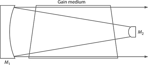
FIGURE 1.15 Basic unstable resonator laser cavity.
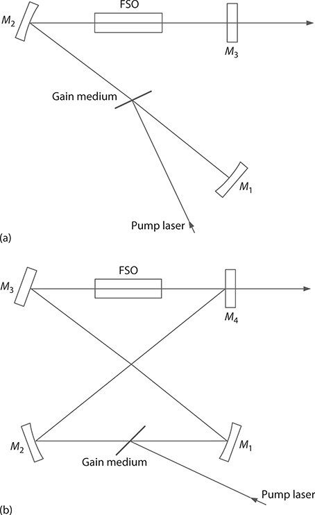
FIGURE 1.16 (a) Linear and (b) unidirectional eight-shaped ring dye laser cavities.
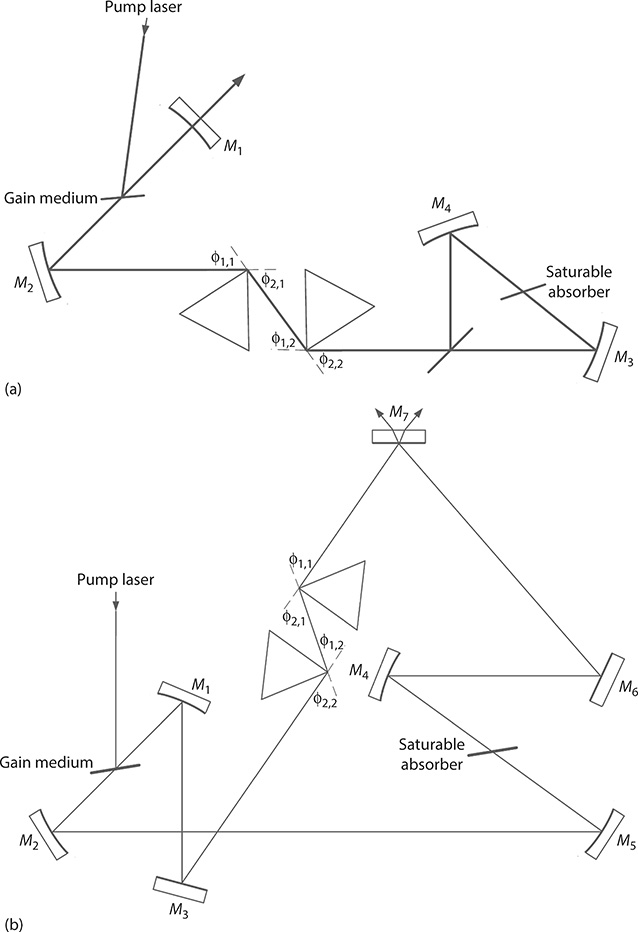
FIGURE 1.17 (a) Linear femtosecond laser cavity. (b) Ring femtosecond laser resonator. Both laser configurations include a saturable absorber and a multiple-prism pulse compressor.
Although most lasers do need efficient and well-designed optical resonators, some lasers have such high gain factors that they tend to emit laser like radiation sometimes called superradiant emission or superfluorescence with only one mirror, or even without external mirrors. This means that the intrinsic reflection factors from flat windows provide the necessary feedback for powerful emission albeit with poor coherence properties. More specifically, this emission tends to be broadband and highly divergent. One additional advantage of using inclined windows, when using high gain laser media, is to reduce parasitic reflections that tend to contribute to output noise. Some laser media that produce very high gains include copper vapor, molecular nitrogen, and laser dyes.
Problems
1.1 Show that in the steady state Equation 1.14 becomes Equation 1.18.
1.2 Show that in the steady state Equation 1.17 becomes Equation 1.21.
1.3 Show that by neglecting the triplet state from Equation 1.21, the gain can be expressed as Equation 1.23.
1.4 Starting from Equations 1.40 and 1.41, derive an expression for |DI|2 and show that it is equal to |DII|2.
1.5 Use Equation 1.53 to arrive at the expression for the transition cross section given in Equation 1.54.
1.6 For a 3 → 2 transition, use Equation 1.99 to estimate the emission wavelength of the GaInAs quantum cascade laser reported by Faist et al. (1994).