Chapter 2 Dirac Optics

Search in book...
Toggle Font Controls
Create new playlist

Name your new playlist

Playlist description (optional)
Sign In

Email address

Password

Forgot Password?

or

Continue with Facebook

Continue with Google
Sign Up

Full Name

Email address

Confirm Email Address

Password

or

Continue with Facebook

Continue with Google

Dirac introduced his enormously practical quantum bra–ket notation in 1939 as a “new notation for quantum mechanics” (Dirac 1939). Also, he discussed in his classic book Principles of Quantum Mechanics, first published in 1930 (Dirac 1978), the essence of interference as a one-photon phenomenon. He did so within a macroscopic framework using concepts such as “a beam of light consisting of a large number of photons,” beam splitters,” and “translational states of a photon” (Dirac 1978). That primordial and illuminating discussion surely qualifies Dirac as the father of quantum optics.

In 1965, Feynman discussed electron interference in two-slit thought experiments using probability amplitudes and Dirac’s notation as tools (Feynman et al. 1965b). In 1991, Dirac’s notation was applied to the propagation of coherent light in an N-slit interferometer (Duarte 1991). The emphasis of this chapter is to provide a straightforward introduction to the description of generalized interference using Dirac’s notation. Here, the content, format, and style follow closely the initial introduction (Duarte 2003), although the discussion is extended using newer material (Duarte 2006) and relevant concepts adopted in a recent review (Duarte 2014).

2.2 Dirac’s Notation in Optics

The concept of the notation invented by Dirac can be explained by considering the propagation of a particle from plane s to plane x, as illustrated in Figure 2.1. According to the Dirac concept, there is a probability amplitude, denoted by 〈x|s〉, that quantifies such propagation. Historically, Dirac introduced the nomenclature of ket vectors, denoted by | 〉, and bra vectors, denoted by 〈 |, which are mirror images of each other. Thus, the probability amplitude is described by the bra–ket 〈x | s〉, which is a complex number.

It is important to note that in Dirac’s notation the propagation from s to x is expressed in reverse by 〈x | s〉. In other words, the starting condition is at the right and the final condition is at the left. If the propagation of the photon is not directly from plane s to plane x, but it involves the passage through an intermediate plane j, as illustrated in Figure 2.2, then the probability amplitude describing such propagation is

〈 x | s 〉 = 〈 x | j 〉 〈 j | s 〉 (2.1)

$〈 x | s 〉 = 〈 x | j 〉 〈 j | s 〉 (2.1)$

If the photon from s must also propagate through planes j and k in its trajectory to x, as illustrated in Figure 2.3, then the probability amplitude is given by

〈 x | s 〉 = 〈 x | k 〉 〈 k | j 〉 〈 j | s 〉 (2.2)

$〈 x | s 〉 = 〈 x | k 〉 〈 k | j 〉 〈 j | s 〉 (2.2)$

Images

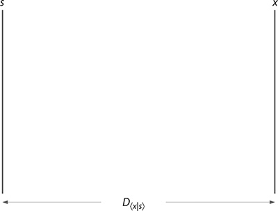
FIGURE 2.1 Propagation from s to x is expressed as 〈x | s〉.

Images

FIGURE 2.2 Propagation from s to x via an intermediate plane j is expressed as 〈x | j〉 〈j | s〉.

Images

FIGURE 2.3 Propagation from s to x via two intermediate planes j and k is expressed as 〈x | k〉 〈k | j〉 〈j | s〉.

When at the intermediate plane of the case in Figure 2.2, a number of alternatives N are available to the passage of the photon, as depicted in Figure 2.4a; the overall probability amplitude must consider every possible alternative, which is expressed mathematically by a summation over j in the form of

〈 x | s 〉 = \sum_{j = 1}^{N} 〈 x | j 〉 〈 j | s 〉 (2.3)

$〈 x | s 〉 = \sum_{j = 1}^{N} 〈 x | j 〉 〈 j | s 〉 (2.3)$

For the case of an additional intermediate plane with N alternatives, as illustrated in Figure 2.4b, the probability amplitude is written as

〈 x | s 〉 = \sum_{k = 1}^{N} \sum_{j = 1}^{N} 〈 x | k 〉 〈 k | j 〉 〈 j | s 〉 (2.4)

$〈 x | s 〉 = \sum_{k = 1}^{N} \sum_{j = 1}^{N} 〈 x | k 〉 〈 k | j 〉 〈 j | s 〉 (2.4)$

Images

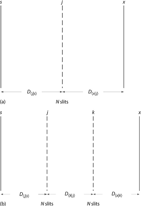
FIGURE 2.4 (a) Propagation from s to x via an array of N slits positioned at the intermediate plane j. (b) Propagation from s to x via an array of N slits positioned at the intermediate plane j and via an additional array of N slits positioned at k.

The addition of further intermediate planes, with N alternatives, can then be systematically incorporated in the notation. The Dirac notation, albeit originally applied to the propagation of a single photon or electron (Dirac 1978; Feynman et al. 1965a), also applies to describe the propagation of ensembles of coherent, or indistinguishable, photons, or indistinguishable quanta (Duarte 1991, 1993). This is in agreement with the interpretation that suggests that the principles of quantum mechanics are applicable to the description of macroscopic phenomena, which are not perturbed by observation (van Kampen 1988).

2.3 Interference

As outlined by Feynman in his thought experiments, on two-slit electron interference, Dirac’s notation offers a natural avenue to describe the propagation of electrons from a source to a detection plane via a pair of slits. This idea can be extended to the description of photon propagation from a source s to a screen detector x, via a transmission grating j comprised by N slits, as illustrated in Figure 2.5.

In the experimental scheme of Figure 2.5, a narrow-linewidth, or highly coherent, laser emits a Gaussian beam that is expanded in one dimension in the plane of propagation, or plane of incidence. Then, the central part of that expanded beam propagates through a wide illumination aperture, thus configuring the radiation source (s) that illuminates an array of N slits, or transmission grating ( j). The interaction of the coherent radiation with the transmission grating ( j) produces an interference signal atx. A crucial point here is that all the indistinguishable photons, or indistinguishable quanta, illuminate the array of N slits, or grating, simultaneously. If only one photon propagates, at any given time, then that individual photon illuminates the whole array of N slits simultaneously. The probability amplitude that describes the propagation from the source (s) to the detection plane (x), via the array of N slits ( j), is given by (Duarte 1991, 1993)

〈 x | s 〉 = \sum_{j = 1}^{N} 〈 x | j 〉 〈 j | s 〉

$〈 x | s 〉 = \sum_{j = 1}^{N} 〈 x | j 〉 〈 j | s 〉$

Images

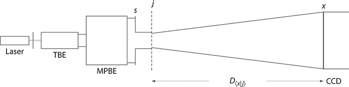
FIGURE 2.5 Optical architecture of the N-slit laser interferometer. Light from a TEM₀₀ narrow-linewidth laser is transformed into an extremely elongated near-Gaussian source (s) to illuminate an array of N slits at j. Interaction of the coherent emission with the slit array produces interference at x. The j-to-x intra-interferometric distance is D_〈x|j〉. This class of interferometric architecture was first introduced by Duarte (1991, 1993). (Reproduced from Duarte, F.J., et al., J. Opt., 12, 015705, 2010. With permission from the Institute of Physics.)

According to Dirac (1978), the probability amplitudes can be represented by wave functions of ordinary wave optics. Thus, following Feynman et al. (1965a),

〈 j | s 〉 = Ψ (r_{j, s}) e^{- i θ_{j}} (2.5)

$〈 j | s 〉 = Ψ (r_{j, s}) e^{- i θ_{j}} (2.5)$

〈 x | j 〉 = Ψ (r_{x, j}) e^{- i ϕ_{j}} (2.6)

$〈 x | j 〉 = Ψ (r_{x, j}) e^{- i ϕ_{j}} (2.6)$

where:

θ_j and ϕ_j are the phase terms associated with the incidence and diffraction waves, respectively

Using these expressions for the probability amplitudes, then, Equation 2.3 can be written as

〈 x | s 〉 = \sum_{j = 1}^{N} Ψ (r_{j}) e^{- l} Ω_{j} (2.7)

$〈 x | s 〉 = \sum_{j = 1}^{N} Ψ (r_{j}) e^{- l} Ω_{j} (2.7)$

where:

Ψ (r_{j}) = Ψ (r_{x, j}) Ψ (r_{j, s}) (2.8)

$Ψ (r_{j}) = Ψ (r_{x, j}) Ψ (r_{j, s}) (2.8)$

and

Ω_{j} = (θ_{j} + (ϕ_{j}) (2.9)

$Ω_{j} = (θ_{j} + (ϕ_{j}) (2.9)$

The propagation probability can be obtained by expanding Equation 2.7 and multiplying the expansion by its complex conjugate. In other words, by performing the multiplication

〈 x | s 〉 〈 x | s 〉^{*} = | 〈 x | s 〉 |^{2} (2.10)

$〈 x | s 〉 〈 x | s 〉^{*} = | 〈 x | s 〉 |^{2} (2.10)$

and using the identity

2 \cos (Ω_{m} - Ω_{j}) = e^{- i (Ω_{m} - Ω_{j})} + e^{i (Ω_{m} - Ω_{j})} (2.11)

$2 \cos (Ω_{m} - Ω_{j}) = e^{- i (Ω_{m} - Ω_{j})} + e^{i (Ω_{m} - Ω_{j})} (2.11)$

we can write the generalized propagation probability in one dimension:

| 〈 x | s 〉 |^{2} = \sum_{j = 1}^{N} Ψ (r_{j}) \sum_{m = 1}^{N} Ψ (r_{m}) e^{i (Ω_{m} - Ω_{j})} (2.12)

$| 〈 x | s 〉 |^{2} = \sum_{j = 1}^{N} Ψ (r_{j}) \sum_{m = 1}^{N} Ψ (r_{m}) e^{i (Ω_{m} - Ω_{j})} (2.12)$

which can be expressed as (Duarte and Paine 1989; Duarte 1991)

| 〈 x | s 〉 |^{2} = \sum_{j = 1}^{N} Ψ (r_{j})^{2} + 2 \sum_{j = 1}^{N} Ψ (r_{j}) (\sum_{m = j + 1}^{N} Ψ (r_{m}) \cos (Ω_{m} - Ω_{j})) (2.13)

$| 〈 x | s 〉 |^{2} = \sum_{j = 1}^{N} Ψ (r_{j})^{2} + 2 \sum_{j = 1}^{N} Ψ (r_{j}) (\sum_{m = j + 1}^{N} Ψ (r_{m}) \cos (Ω_{m} - Ω_{j})) (2.13)$

Interference due to transmission in a two-dimensional transmission grating can be described considering the experimental setup depicted in Figure 2.6. Propagation of quanta occurs from s to x via a two-dimensional transmission grating j_zy, that is, j is replaced by a grid comprising j components in the y direction and j components in the z direction. Note that in the one-dimensional case, only the y component of j is present, which is written simply as j. The plane configured by the j_zy grid is orthogonal to the plane of propagation. Hence, for photon propagation from s to x, via j_zy, the probability amplitude is given by (Duarte 1995a)

Images

FIGURE 2.6 A two-dimensional representation of the 〈x | j〉 〈j | s〉 geometry.

〈 x | s 〉 = \sum_{j_{Z} = 1}^{N} \sum_{j_{y} = 1}^{N} 〈 x | j_{z y} 〉 〈 j_{z y} | s 〉 (2.14)

$〈 x | s 〉 = \sum_{j_{Z} = 1}^{N} \sum_{j_{y} = 1}^{N} 〈 x | j_{z y} 〉 〈 j_{z y} | s 〉 (2.14)$

Now, if j is abstracted from j_zy, then the above equation can be expressed as

〈 x | s 〉 = \sum_{z = 1}^{N} \sum_{y = 1}^{N} Ψ (r_{z y}) e^{- l} Ω_{z y} (2.15)

$〈 x | s 〉 = \sum_{z = 1}^{N} \sum_{y = 1}^{N} Ψ (r_{z y}) e^{- l} Ω_{z y} (2.15)$

and the corresponding probability is given by (Duarte 1995a)

| 〈 x | s 〉 |^{2} = \sum_{z = 1}^{N} \sum_{y = 1}^{N} Ψ (r_{z y}) \sum_{q = 1}^{N} \sum_{p = 1}^{N} Ψ (r_{q p}) e^{i (Ω_{q p} - Ω_{z y})} (2.16)

$| 〈 x | s 〉 |^{2} = \sum_{z = 1}^{N} \sum_{y = 1}^{N} Ψ (r_{z y}) \sum_{q = 1}^{N} \sum_{p = 1}^{N} Ψ (r_{q p}) e^{i (Ω_{q p} - Ω_{z y})} (2.16)$

For a three-dimensional transmission grating, it can be shown that (Duarte 1995a)

| 〈 x | s 〉 |^{2} = \sum_{z = 1}^{N} \sum_{y = 1}^{N} \sum_{x = 1}^{N} Ψ (r_{z y x}) \sum_{q = 1}^{N} \sum_{p = 1}^{N} \sum_{r = 1}^{N} Ψ (r_{q p r}) e^{i (Ω_{q p} \cdot - Ω_{z y x})} l (2.17)

$| 〈 x | s 〉 |^{2} = \sum_{z = 1}^{N} \sum_{y = 1}^{N} \sum_{x = 1}^{N} Ψ (r_{z y x}) \sum_{q = 1}^{N} \sum_{p = 1}^{N} \sum_{r = 1}^{N} Ψ (r_{q p r}) e^{i (Ω_{q p} \cdot - Ω_{z y x})} l (2.17)$

It is important to emphasize that the concepts described here apply to either the propagation of single photons and the propagation of ensembles of coherent, indistinguishable, or monochromatic photons or quanta. The application of quantum principles to the description of propagation of a large number of monochromatic, or indistinguishable, photons was already advanced by Dirac in his discussion of interference (Dirac 1978; Duarte 1998).

2.3.1 Example

The generalized interference equation in one dimension (Equation 2.13) can be used to write explicit expressions for double-slit (N = 2), triple-slit (N = 3), quadruple-slit (N = 4), quintuple-slit (N = 5), sextuple-slit (N = 6), septuple-slit (N = 7) interference, and so on. For a seven-slit (N = 7) interference, we get

\begin{matrix} | 〈 x | s 〉 |^{2} = Ψ (r)^{2} + Ψ (r_{2})^{2} + Ψ (r_{3})^{2} + Ψ (r_{4})^{2} + Ψ (r_{5})^{2} + Ψ (r_{6})^{2} + Ψ (r_{7})^{2} \\ + 2 [Ψ (r) Ψ (r_{2}) \cos (Ω_{2} - Ω_{1}) + Ψ (r) Ψ (r_{3}) \cos (Ω_{3} - Ω_{1}) + Ψ (r) Ψ (r_{4}) \cos (Ω_{4} - Ω_{1}) \\ + Ψ (r) Ψ (r_{5}) \cos (Ω_{5} - Ω_{1}) + Ψ (r) Ψ (r_{6}) \cos (Ω_{6} - Ω_{1}) + Ψ (r) Ψ (r_{7}) \cos (Ω_{7} - Ω_{1}) \\ + Ψ (r_{2}) Ψ (r_{3}) \cos (Ω_{3} - Ω_{2}) + Ψ (r_{2}) Ψ (r_{4}) \cos (Ω_{4} - Ω_{2}) + Ψ (r_{2}) Ψ (r_{5}) \cos (Ω_{5} - Ω_{2}) \\ + Ψ (r_{2}) Ψ (r_{6}) \cos (Ω_{6} - Ω_{2}) + Ψ (r_{2}) Ψ (r_{7}) \cos (Ω_{7} - Ω_{2}) + Ψ (r_{3}) Ψ (r_{4}) \cos (Ω_{4} - Ω_{3}) \\ + Ψ (r_{3}) Ψ (r_{5}) \cos (Ω_{5} - Ω_{3}) + Ψ (r_{3}) Ψ (r_{6}) \cos (Ω_{6} - Ω_{3}) + Ψ (r_{3}) Ψ (r_{7}) \cos (Ω_{7} - Ω_{3}) \\ + Ψ (r_{4}) Ψ (r_{5}) \cos (Ω_{5} - Ω_{4}) + Ψ (r_{4}) Ψ (r_{6}) \cos (Ω_{6} - Ω_{4}) + Ψ (r_{4}) Ψ (r_{7}) \cos (Ω_{7} - Ω_{4}) \\ + Ψ (r_{5}) Ψ (r_{6}) \cos (Ω_{6} - Ω_{5}) + Ψ (r_{5}) Ψ (r_{7}) \cos (Ω_{7} - Ω_{5}) + Ψ (r_{6}) Ψ (r_{7}) \cos (Ω_{7} - Ω_{6})] \end{matrix} (2.18)

$\begin{matrix} | 〈 x | s 〉 |^{2} = Ψ (r)^{2} + Ψ (r_{2})^{2} + Ψ (r_{3})^{2} + Ψ (r_{4})^{2} + Ψ (r_{5})^{2} + Ψ (r_{6})^{2} + Ψ (r_{7})^{2} \\ + 2 [Ψ (r) Ψ (r_{2}) \cos (Ω_{2} - Ω_{1}) + Ψ (r) Ψ (r_{3}) \cos (Ω_{3} - Ω_{1}) + Ψ (r) Ψ (r_{4}) \cos (Ω_{4} - Ω_{1}) \\ + Ψ (r) Ψ (r_{5}) \cos (Ω_{5} - Ω_{1}) + Ψ (r) Ψ (r_{6}) \cos (Ω_{6} - Ω_{1}) + Ψ (r) Ψ (r_{7}) \cos (Ω_{7} - Ω_{1}) \\ + Ψ (r_{2}) Ψ (r_{3}) \cos (Ω_{3} - Ω_{2}) + Ψ (r_{2}) Ψ (r_{4}) \cos (Ω_{4} - Ω_{2}) + Ψ (r_{2}) Ψ (r_{5}) \cos (Ω_{5} - Ω_{2}) \\ + Ψ (r_{2}) Ψ (r_{6}) \cos (Ω_{6} - Ω_{2}) + Ψ (r_{2}) Ψ (r_{7}) \cos (Ω_{7} - Ω_{2}) + Ψ (r_{3}) Ψ (r_{4}) \cos (Ω_{4} - Ω_{3}) \\ + Ψ (r_{3}) Ψ (r_{5}) \cos (Ω_{5} - Ω_{3}) + Ψ (r_{3}) Ψ (r_{6}) \cos (Ω_{6} - Ω_{3}) + Ψ (r_{3}) Ψ (r_{7}) \cos (Ω_{7} - Ω_{3}) \\ + Ψ (r_{4}) Ψ (r_{5}) \cos (Ω_{5} - Ω_{4}) + Ψ (r_{4}) Ψ (r_{6}) \cos (Ω_{6} - Ω_{4}) + Ψ (r_{4}) Ψ (r_{7}) \cos (Ω_{7} - Ω_{4}) \\ + Ψ (r_{5}) Ψ (r_{6}) \cos (Ω_{6} - Ω_{5}) + Ψ (r_{5}) Ψ (r_{7}) \cos (Ω_{7} - Ω_{5}) + Ψ (r_{6}) Ψ (r_{7}) \cos (Ω_{7} - Ω_{6})] \end{matrix} (2.18)$

2.3.2 Geometry of The N-Slit Interferometer

In addition to the generalized interferometric equations, it is important to consider the geometry of the transmission grating ( j) in conjunction with the plane of interference (x) for the one-dimensional case as illustrated in Figure 2.7. According to the geometry, the phase difference term in Equation 2.13 can be expressed as (Duarte 1997)

\cos [(θ_{m} - θ_{j}) \pm (ϕ_{m} - ϕ_{j})] = \cos (| l_{m} - l_{m - 1} | k_{1} \pm | L_{m} - L_{m - 1} | k_{2}) (2.19)

$\cos [(θ_{m} - θ_{j}) \pm (ϕ_{m} - ϕ_{j})] = \cos (| l_{m} - l_{m - 1} | k_{1} \pm | L_{m} - L_{m - 1} | k_{2}) (2.19)$

where:

k_{1} = \frac{2 π n_{1}}{λ_{v}} (2.20)

$k_{1} = \frac{2 π n_{1}}{λ_{v}} (2.20)$

and

k_{2} = \frac{2 π n_{2}}{λ_{v}} (2.21)

$k_{2} = \frac{2 π n_{2}}{λ_{v}} (2.21)$

Images

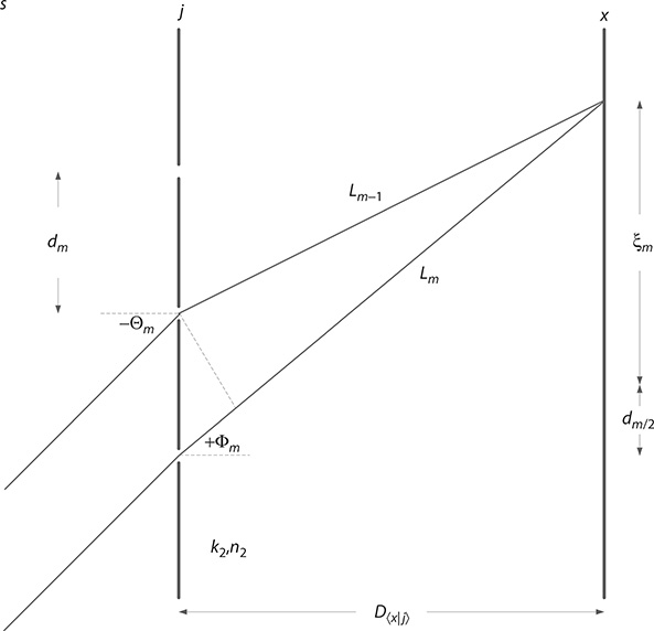
FIGURE 2.7 A detailed representation of the 〈x | j〉 〈j | s〉 geometry depicting the difference in path length and the angles of incidence and diffraction. (Reproduced from Duarte, F.J., Am. J. Phys., 65, 637–640, 1997. With permission from the American Association of Physics Teachers.)

are the wavenumbers of the two optical regions defined in Figure 2.7. Here, λ₁ = λ_v/n₁ and λ₂ = λ_v/n₂, where λ_v is the vacuum wavelength and n₁ and n₂ are the corresponding indexes of refraction (Wallenstein and Hänsch 1974; Born and Wolf 1999). The phase differences can be expressed exactly via the following geometrical equations (Duarte 1993):

| L_{m} - L_{m - 1} | = \frac{2 ξ_{m} d_{m}}{| L_{m} + L_{m - 1} |} (2.22)

$| L_{m} - L_{m - 1} | = \frac{2 ξ_{m} d_{m}}{| L_{m} + L_{m - 1} |} (2.22)$

L_{m}^{2} = D_{〈 x | j 〉}^{2} + (ξ_{m} + \frac{d_{m}}{2})^{2} (2.23)

$L_{m}^{2} = D_{〈 x | j 〉}^{2} + (ξ_{m} + \frac{d_{m}}{2})^{2} (2.23)$

L_{m - 1}^{2} = D_{〈 x | j 〉}^{2} + (ξ_{m} - \frac{d_{m}}{2})^{2} (2.24)

$L_{m - 1}^{2} = D_{〈 x | j 〉}^{2} + (ξ_{m} - \frac{d_{m}}{2})^{2} (2.24)$

In this notation, ξ_m is the lateral displacement, on the x plane, from the projected median of d_m to the interference plane.

2.3.3 N-Slit Interferometer Experiment

The N-slit interferometer is illustrated in Figure 2.5. In practice, this interferometer can be configured with a variety of lasers including tunable lasers. However, one requirement is that the laser to be utilized must emit in the narrow-linewidth regime and in a single transverse mode (TEM₀₀) with a near-Gaussian profile. Ideally, the source should be a single-longitudinal-mode laser. The reason for this requirement is that narrow-linewidth lasers yield sharp, well-defined interference patterns close to those predicted theoretically for a single wavelength.

One particular configuration of the N-slit interferometer can be integrated by a TEM₀₀ He–Ne laser (λ = 632.82 nm) with a beam 0.5 mm in diameter. It should be emphasized that this class of laser yields a smooth near-Gaussian beam profile and narrow-linewidth emission. The laser beam is then magnified, in two dimensions, by a ×20 Galilean telescope. Following the telescopic expansion, the beam is further expanded in one dimension by a ×5 multiple-prism beam expander. This optical arrangement yields an expanded smooth near-Gaussian beam approximately 50 mm wide. An option is to insert a convex lens prior to the multiple-prism expander. This produces an extremely elongated near-Gaussian beam of 20–30 μm at it maximum height by 50 mm in width (Duarte 1993). The beam propagation through this system can be accurately characterized using ray transfer matrices as discussed in Chapter 6 (Duarte 1995b). Also, as an option, at the exit of the multiple-prism beam expander, an aperture, a few millimeters wide, can be deployed. Thus, the source s can be either the exit prism of the multiple-prism beam expander or the wide aperture.

At this stage, it should be noted that for the illumination of two slits 50 μm in width, separated by 50 μm, the elongated Gaussian provides a nearly plane illumination profile, which is also approximately the case even if a larger number of slits, of these dimensions, are illuminated. For the particular case of a two-slit experiment, or Young’s interference experiment, involving 50-μm slits separated by 50 μm and a grating-to-screen distance (a) of 10 cm, the interference signal is displayed in Figure 2.8a. The calculated interference using Equation 2.13 and assuming plane wave illumination is given in Figure 2.8b. The interference screen at x is a digital detector comprising a photodiode array, each 25 μm in width. For an array of N = 100 slits, each 30 μm in width and separated by 30 μm, the measured and calculated interferograms are shown in Figure 2.9. Here, the grating-to-digital detector distance is D_{〈x | j〉} = 75 cm.

In practice, the transmission gratings are not perfect and offer an uncertainty in the dimension of the slits. The uncertainty in the slit dimensions of the grating, incorporating the 30-μm slits, used in this experiment was measured to be ≤2%. The theoretical interferogram for the grating comprising N = 100 slits, each 30.0 ± 0.6 μm wide and separated by 30.0 ± 0.6 μm, is given in Figure 2.10. Notice the slight symmetry deterioration.

When a wide slit is used to select the central portion of the elongated Gaussian beam, the interaction of the coherent laser beam with the slit results in diffraction prior to the illumination of the transmission grating. The interferometric equation (2.13) can be used to characterize this diffraction. This is done by dividing the wide slit into hundreds of smaller slits. As an example, a 4-mm-wide aperture is divided into 800 slits, each 4 μm wide and separated by a 1-μm interslit distance. The calculated near-field diffraction pattern, for a distance on intra-interferometric distance of D_{〈x | j〉} = 10 cm, is shown in Figure 2.11. Using this as the radiation source to illuminate the 100-slit grating, comprising 30 μm slits with an interslit distance of 30 μm (for D_{〈x | j〉} = 75 cm), yields the theoretical interferogram displayed in Figure 2.12. Thus, the interferometric equation (2.13) can be used in a cascade approach from an illumination plane to an interference plane. This cascade approach can be applied to multiple intermediate planes. More on this approach is given in Chapter 10.

Images

FIGURE 2.8 (a) Measured interferogram resulting from the interaction of coherent laser emission at λ = 632.82 nm and two (N = 2) slits 50 μm wide, separated by 50 μm. The j-to-x distance is D_{〈x | j〉} = 10 cm. (b) Corresponding theoretical interferogram from Equation 2.13. Note that the screen axial distance refers to the distance at the interferometric plane that defines the spatial width of the interferogram and that is perpendicular to the propagation axis. (Reproduced from Duarte, F.J., Quantum Optics for Engineers, CRC Press, New York, 2014. With permission from Taylor & Francis.)

Images

FIGURE 2.9 (a) Measured interferogram resulting from the interaction of coherent laser emission at λ = 632.82 nm and N = 100 slits 30 μm wide, separated by 30 μm. The j-to-x distance is D_{〈x | j〉} = 75 cm. (b) Corresponding theoretical interferogram from Equation 2.13. (Reprinted from Opt. Commun., 103, Duarte, F.J., On a generalized interference equation and interferometric measurements, 8–14, Copyright 1993, with permission from Elsevier.)

Images

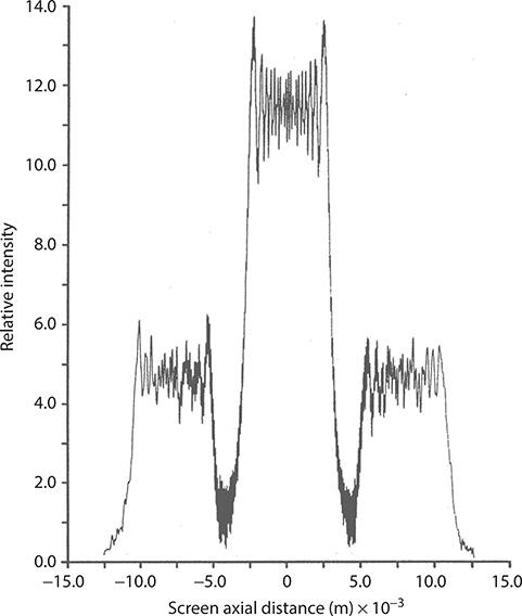
FIGURE 2.10 Theoretical interferometric/diffraction distribution using a ≤2% uncertainty in the dimensions of the 30-μm slits. In this calculation, N = 100 and the j-to-x distance is D_{〈x | j〉} = 75 cm. A slight deterioration in the spatial symmetry of the distribution is evident. (Reprinted from Opt. Commun., 103, Duarte, F.J., On a generalized interference equation and interferometric measurements, 8–14, Copyright 1993, with permission from Elsevier.)

2.4 Generalized Diffraction

Feynman, in his usual style, stated that “no one has ever been able to define the difference between interference and diffraction satisfactorily” (Feynman et al. 1965b; pp. 30–1). His point is well taken. In the discussion related to Figure 2.9, and its variants, reference was only made to interference. However, what we really have is interference in three diffraction orders: the zeroth, or central order, and the ±1, or secondary orders. In other words, there is an interference pattern associated with each diffraction order. Physically, however, it is the same phenomenon. The interaction of coherent light with a set of slits, in the near field, gives rise to an interference pattern. As the distance D_{〈x | j〉} from j to x increases, the central interference pattern begins to give origin to secondary patterns that gradually separate from the central order at lower intensities. These are the ±1 diffraction orders. This physical phenomenon, as one goes from the near to the far field, is illustrated in Figure 2.13. One of the beauties of the Dirac description of optics is the ability to continuously move from the near to the far field with a single mathematical description.

Images

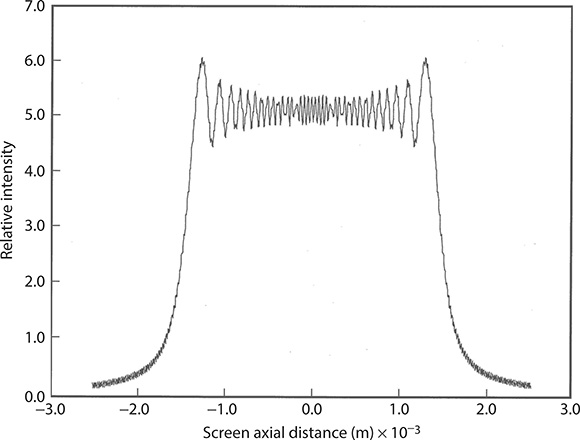
FIGURE 2.11 Theoretical near-field diffraction distribution produced by a 4-mm aperture illuminated at λ = 632.82 nm. The j-to-x distance is D_{〈x | j〉} = 10 cm. (Reprinted from Opt. Commun., 103, Duarte, F.J., On a generalized interference equation and interferometric measurements, 8–14, Copyright 1993, with permission from Elsevier.)

The second interference–diffraction entanglement refers to the fact that our generalized interference equation can be naturally applied to describe a diffraction pattern produced by a single wide slit as shown in Figure 2.11. Under these circumstances, the wide slit is mathematically represented by a series of subslits.

The generalized description of diffraction given next includes the refinement and extension of the original presentation given by Duarte (1997, 2003) and includes the treatment of positive and negative diffraction as introduced by Duarte (2006), and follows the style of Duarte (2014).

The intimate relation between interference and diffraction has its origin in the interferometric equation itself (Duarte 2003):

| 〈 x | s 〉 |^{2} = \sum_{j = 1}^{N} Ψ (r_{j})^{2} + 2 \sum_{j = 1}^{N} Ψ (r_{j}) [\sum_{m = j + 1}^{N} Ψ (r_{m}) \cos (Ω_{m} - Ω_{j})]

$| 〈 x | s 〉 |^{2} = \sum_{j = 1}^{N} Ψ (r_{j})^{2} + 2 \sum_{j = 1}^{N} Ψ (r_{j}) [\sum_{m = j + 1}^{N} Ψ (r_{m}) \cos (Ω_{m} - Ω_{j})]$

for it is the cos(Ω_m - Ω_j) term that gives rise to different diffraction orders while the interference follows the mechanics established the overall equation. Here, we revisit the geometry at the N-slit plane j and illustrate what is obviously seen in Figure 2.13: up on arrival to a slit, diffraction occurs symmetrically toward both sides as illustrated in Figures 2.14 through 2.17. Figure 2.14 depicts the usual description associated with incidence below the normal (−) and diffraction above the normal (+). Figure 2.15 illustrates the incidence above the normal (+) and the diffraction above the normal (+) (Duarte 2006). For completeness, we also include the case of incidence below the normal (−) followed by diffraction below the normal (−) and incidence above the normal (+) followed by diffraction below the normal (−) (Figures 2.16 and 2.17). Thus, the equations describing the original geometry (Duarte 1997) are slightly modified to account for all the ± alternatives:

Images

FIGURE 2.12 Theoretical interferometric distribution illustrating a cascade calculation. It incorporates diffraction-edge effects in the illumination. In this calculation, the width of the slits in the array is 30 μm separated by 30 μm, N = 100, and the j-to-x distance is D_{〈x | j〉} = 75 cm. The aperture-to-grating distance is 10 cm. (Reprinted from Opt. Commun., 103, Duarte, F.J., On a generalized interference equation and interferometric measurements, 8–14, Copyright 1993, with permission from Elsevier.)

\cos [\pm (θ_{m} - θ_{j}) \pm (ϕ_{m} - ϕ_{j})] = \cos (\pm | l_{m} - l_{m - 1} | k_{1} \pm | L_{m} - L_{m - 1} | k_{2}) (2.25)

$\cos [\pm (θ_{m} - θ_{j}) \pm (ϕ_{m} - ϕ_{j})] = \cos (\pm | l_{m} - l_{m - 1} | k_{1} \pm | L_{m} - L_{m - 1} | k_{2}) (2.25)$

where:

k_{1} = \frac{2 π n_{1}}{λ_{v}} (2.26)

$k_{1} = \frac{2 π n_{1}}{λ_{v}} (2.26)$

Images

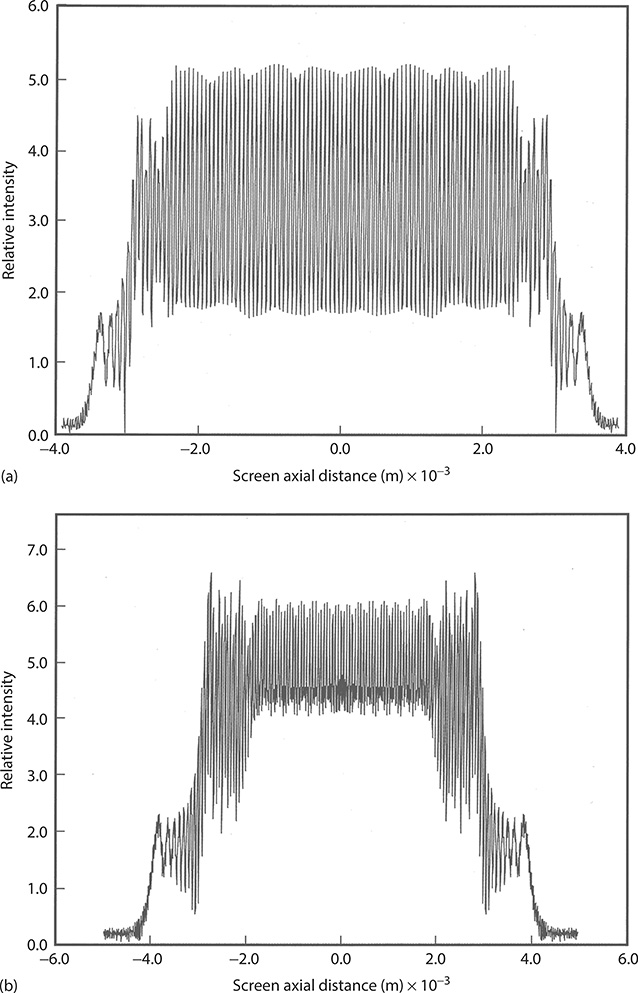
FIGURE 2.13 Emergence of secondary diffraction (±1) orders as the j-to-x distance is increased. (a) At a grating-to-screen distance of D_{〈x | j〉} = 5cm, the interferometric distribution is mainly part of a single order. At the boundaries, there is an incipient indication of emerging orders. (b) As the distance is increased to D_{〈x | j〉} = 10 cm, the presence of the emerging (±1) orders is more visible. (c) At a distance of D_{〈x | j〉} = 25 cm, the emerging (±1) orders give rise to an overall distribution with clear shoulders. (d) At a distance of D_{〈x | j〉} = 75 cm, the −1, 0, and +1 diffraction orders are clearly established. Notice the increase in the width of the distribution as the intra-interferometric distance D_{〈x | j〉} increases from 5 to 75 cm. The width of the slits is 30 μm separated by 30 μm, N = 100, and λ = 632.82 nm.

Images

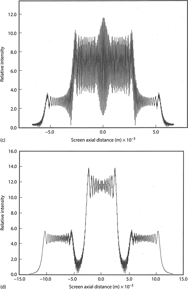
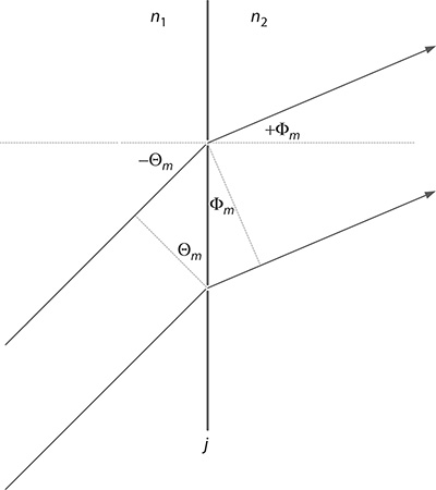
Figure 2.14 Incidence below the normal (−) and diffraction above the normal (+). (Reproduced from Duarte, F.J., Quantum Optics for Engineers, CRC Press, New York, 2014. With permission from Taylor & Francis.)

Images

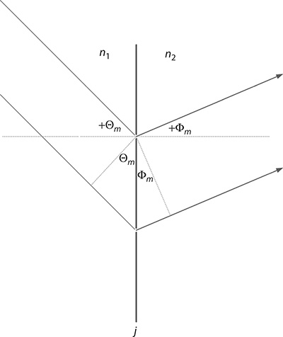
FIGURE 2.15 Incidence above the normal (+) and diffraction above the normal (+). (Reproduced from Duarte, F.J., Quantum Optics for Engineers, CRC Press, New York, 2014. With permission from Taylor & Francis.)

Images

FIGURE 2.16 Incidence below the normal (−) followed by diffraction below the normal (−). (Reproduced from Duarte, F.J., Quantum Optics for Engineers, CRC Press, New York, 2014. With permission from Taylor & Francis.)

Images

FIGURE 2.17 Incidence above the normal (+) followed by diffraction below the normal (−). (Reproduced from Duarte, F.J., Quantum Optics for Engineers, CRC Press, New York, 2014. With permission from Taylor & Francis.)

and

k_{2} = \frac{2 π n_{2}}{λ_{v}} (2.27)

$k_{2} = \frac{2 π n_{2}}{λ_{v}} (2.27)$

are the wavenumbers of the two optical regions defined in Figures 2.14 through 2.17. Here, as we saw earlier, λ₁ = λ_v/n₁ and λ₂ = λ_v/n₂, where λ_v is the vacuum wavelength and n₁ and n₂ are the corresponding indexes of refraction.

As mentioned earlier, the phase differences can be expressed exactly via the exact geometrical expressions (Duarte 1993):

| L_{m} - L_{m - 1} | = \frac{2 ξ_{m} d_{m}}{| L_{m} + L_{m - 1} |} (2.28)

$| L_{m} - L_{m - 1} | = \frac{2 ξ_{m} d_{m}}{| L_{m} + L_{m - 1} |} (2.28)$

L_{m}^{2} = D_{〈 x | j 〉}^{2} + (ξ_{m} + \frac{d_{m}}{2})^{2} (2.29)

$L_{m}^{2} = D_{〈 x | j 〉}^{2} + (ξ_{m} + \frac{d_{m}}{2})^{2} (2.29)$

L_{m - 1}^{2} = D_{〈 x | j 〉}^{2} + (ξ_{m} - \frac{d_{m}}{2})^{2} (2.30)

$L_{m - 1}^{2} = D_{〈 x | j 〉}^{2} + (ξ_{m} - \frac{d_{m}}{2})^{2} (2.30)$

From the geometry of Figure 2.7, we can write

\sin Φ_{m} = \frac{ξ_{m} + (d_{m} / 2)}{L_{m}} (2.31)

$\sin Φ_{m} = \frac{ξ_{m} + (d_{m} / 2)}{L_{m}} (2.31)$

and for the condition D_{〈x | j〉} ≫ d_m, we have |L_m + L_m−1 ≈ 2L_m. Then using Equation 2.28, we have

| L_{m} - L_{m - 1} | \approx d_{m} \sin Φ_{m} (2.32)

$| L_{m} - L_{m - 1} | \approx d_{m} \sin Φ_{m} (2.32)$

| l_{m} - l_{m - 1} | \approx d_{m} \sin Θ_{m} (2.33)

$| l_{m} - l_{m - 1} | \approx d_{m} \sin Θ_{m} (2.33)$

where:

Θ_m and Φ_m are the angles of incidence and diffraction, respectively. Given that maxima occur at

(\pm | l_{m} - l_{m - 1} | n_{1} \pm | L_{m} - L_{m - 1} | n_{2}) \frac{2 π}{λ_{v}} = M π (2.34)

$(\pm | l_{m} - l_{m - 1} | n_{1} \pm | L_{m} - L_{m - 1} | n_{2}) \frac{2 π}{λ_{v}} = M π (2.34)$

then using Equations 2.32 and 2.33

d_{m} (\pm n_{1} \sin Θ_{m} \pm n_{2} \sin Φ_{m}) \frac{2 π}{λ_{v}} = M π (2.35)

$d_{m} (\pm n_{1} \sin Θ_{m} \pm n_{2} \sin Φ_{m}) \frac{2 π}{λ_{v}} = M π (2.35)$

where:

M = 0, 2, 4, 6,...

For n₁ = n₂, we have λ = λ_v, and this equation reduces to the generalized diffraction grating equation:

d_{m} (\pm \sin Θ_{m} \pm \sin Φ_{m}) = m λ (2.36)

$d_{m} (\pm \sin Θ_{m} \pm \sin Φ_{m}) = m λ (2.36)$

where:

m = 0, 1, 2, 3,... are the various diffraction orders

A most important observation is due here: in our discussion on the interferometric equations, we have made explicit reference to the exact geometrical equations (2.28 through 2.30). However, in the derivation of Equations 2.35 and 2.36, we have used the approximation D_{〈x | j〉} ≫ d_m. Are we being consistent? The answer is yes. The exact equations (2.28 through 2.30) are used in the generalized interferometric equation (2.13), whereas the approximation D_{〈x | j〉} ≫ d_m has been applied in the derivation of the generalized diffraction equation

d_{m} (\pm \sin Θ_{m} \pm \sin Φ_{m}) = m λ

$d_{m} (\pm \sin Θ_{m} \pm \sin Φ_{m}) = m λ$

that manifests itself in the far field as beautifully illustrated in Figure 2.13d. From Equation 2.36, it is clearly seen that beyond the zeroth order, m can take a series of ± values, that is, m = ±1, ±2, ±3,... .

2.4.1 Positive Diffraction

From the generalized diffraction equation (2.36) including both ± alternatives, the usual traditional diffraction equation can be stated as

d_{m} (\sin Θ_{m} \pm \sin Φ_{m}) = m λ (2.37)

$d_{m} (\sin Θ_{m} \pm \sin Φ_{m}) = m λ (2.37)$

which was previously derived starting from (Duarte 1997)

\cos [(θ_{m} - θ_{j}) \pm ((ϕ_{m} - (ϕ_{j})] = \cos (| l_{m} - l_{m - 1} | k_{1} \pm | L_{m} - L_{m - 1} | k_{2}) (2.38)

$\cos [(θ_{m} - θ_{j}) \pm ((ϕ_{m} - (ϕ_{j})] = \cos (| l_{m} - l_{m - 1} | k_{1} \pm | L_{m} - L_{m - 1} | k_{2}) (2.38)$

From Equation 2.37, setting Θ_m = Φ_m = Θ, the diffraction grating equation for Littrow configuration emerges from the well-known grating equation:

m λ = 2 d_{m} \sin Θ (2.39)

$m λ = 2 d_{m} \sin Θ (2.39)$

2.5 Positive and Negative Refraction

So far we have discussed interference and diffraction and we have seen how diffraction manifests itself as the interferometric distribution propagates toward the far field. An additional fundamental phenomenon in optics is refraction.

Refraction is the change in the geometrical path of a beam of light due to transmission from the original medium of propagation to a second medium with a different refractive index. For example, refraction is the bending of a ray of light caused due to propagation in a glass, or crystalline, prism.

If in the diffraction grating equation d_m is made very small relative to a given λ, diffraction ceases to occur and the only solution can be found for m = 0 (Duarte 1997). That is, under these conditions, a grating made of grooves coated on a transparent substrate, such as optical glass, does not diffract but exhibits the refraction properties of the glass. For example, since the maximum value of (±sin Θ_m ±sin Φ_m) is 2, for a 5000-lines/mm transmission grating, let us say, no diffraction can be observed for the visible spectrum. Hence, for the condition d_m ≪ λ, the diffraction grating equation can only be solved for

d_{m} (\pm n_{1} \sin Θ_{m} \pm n_{2} \sin Φ_{m}) \frac{2 π}{λ_{v}} = 0 (2.40)

$d_{m} (\pm n_{1} \sin Θ_{m} \pm n_{2} \sin Φ_{m}) \frac{2 π}{λ_{v}} = 0 (2.40)$

which leads to

(\pm n_{1} \sin Θ_{m} \pm n_{2} \sin Φ_{m}) = 0 (2.41)

$(\pm n_{1} \sin Θ_{m} \pm n_{2} \sin Φ_{m}) = 0 (2.41)$

For the case of incidence below the normal (−) and refraction above the normal (+) (Figure 2.14),

- n_{1} \sin Θ_{m} + n_{2} \sin Φ_{m} = 0 (2.42)

$- n_{1} \sin Θ_{m} + n_{2} \sin Φ_{m} = 0 (2.42)$

so that

n_{1} \sin Θ_{m} = n_{2} \sin Φ_{m} (2.43)

$n_{1} \sin Θ_{m} = n_{2} \sin Φ_{m} (2.43)$

which is the well-known equation of refraction, also known as Snell’s law. Under the present physical conditions, Θ_m is the angle of incidence and Φ_m becomes the angle of refraction. The same outcome is obtained for incidence above the normal (+) and refraction below the normal (−) (Figure 2.17).

For the case of incidence above the normal (+) and refraction above the normal (+) (Figure 2.15),

+ n_{1} \sin Θ_{m} + n_{2} \sin Φ_{m} = 0 (2.44)

$+ n_{1} \sin Θ_{m} + n_{2} \sin Φ_{m} = 0 (2.44)$

so that

n_{1} \sin Θ_{m} = - n_{2} \sin Φ_{m} (2.45)

$n_{1} \sin Θ_{m} = - n_{2} \sin Φ_{m} (2.45)$

which is the refraction law for negative refraction. The same outcome is obtained for incidence below the normal (−) and diffraction below the normal (−) (Figure 2.16).

2.6 Reflection

The discussion on interference, up to now, has involved an N-slit array or a transmission grating. It should be indicated that the arguments and physics apply equally well to a reflection interferometer (Duarte 2003), that is, to an interferometer incorporating a reflection, rather than a transmission, grating. Explicitly, if a mirror is placed at an infinitesimal distance immediately behind the N-slit array, as illustrated in Figure 2.18, then the transmission interferometer becomes a reflection interferometer. Under these circumstances, the equations

Images

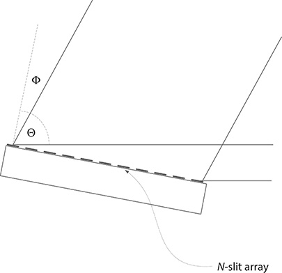
FIGURE 2.18 A reflection diffraction grating is formed by approaching a reflection surface at an infinitesimal distance to the array of N-slits.

d_{m} (\pm n_{1} \sin Θ_{m} \pm n_{2} \sin Φ_{m}) \frac{2 π}{λ_{v}} = M π

$d_{m} (\pm n_{1} \sin Θ_{m} \pm n_{2} \sin Φ_{m}) \frac{2 π}{λ_{v}} = M π$

and

d_{m} (\pm \sin Θ_{m} \pm \sin Φ_{m}) = m λ

$d_{m} (\pm \sin Θ_{m} \pm \sin Φ_{m}) = m λ$

apply in the reflection domain, with Θ_m being the incidence angle and Φ_m the diffraction angle in the reflection domain. For the case of d_m ≪ λ and n₁ = n₂, we then have

(\pm \sin Θ_{m} \pm \sin Φ_{m}) = 0 (2.46)

$(\pm \sin Θ_{m} \pm \sin Φ_{m}) = 0 (2.46)$

For incidence above the normal (+), and reflection below the normal (−),

+ \sin Θ_{m} - \sin Φ_{m} = 0 (2.47)

$+ \sin Θ_{m} - \sin Φ_{m} = 0 (2.47)$

which means

Θ_{m} = Φ_{m} (2.48)

$Θ_{m} = Φ_{m} (2.48)$

where:

Θ_m is the angle of incidence

Φ_m is the angle of reflection

This is known as the law of reflection.

2.7 The Cavity Linewidth Equation

As previously outlined, starting from the generalized interferometric equation

| 〈 x | s 〉 |^{2} = \sum_{j = 1}^{N} Ψ (r_{j})^{2} + 2 \sum_{j = 1}^{N} Ψ (r_{j}) [\sum_{m = j + 1}^{N} Ψ (r_{m}) \cos (Ω_{m} - Ω_{j})]

$| 〈 x | s 〉 |^{2} = \sum_{j = 1}^{N} Ψ (r_{j})^{2} + 2 \sum_{j = 1}^{N} Ψ (r_{j}) [\sum_{m = j + 1}^{N} Ψ (r_{m}) \cos (Ω_{m} - Ω_{j})]$

the generalized diffraction equation

d_{m} (\pm \sin Θ_{m} \pm \sin Φ_{m}) = m λ

$d_{m} (\pm \sin Θ_{m} \pm \sin Φ_{m}) = m λ$

is obtained, and for positive diffraction and Θ_m ≈ Φ_m(= Θ), the diffraction grating equation

2 d \sin Θ = m λ

$2 d \sin Θ = m λ$

in Littrow configuration can be established.

Following the approach of Duarte (1992) and considering two slightly different wavelengths, an expression for the wavelength difference can be written as

Δ λ = \frac{2 d}{m} (\sin Θ_{1} - \sin Θ_{2}) (2.49)

$Δ λ = \frac{2 d}{m} (\sin Θ_{1} - \sin Θ_{2}) (2.49)$

For Θ₁ ≈ Θ₂(= Θ), this equation can be restated as

Δ λ \approx \frac{2 d}{m} Δ θ (1 - \frac{3 Θ^{2}}{3!} + \frac{5 Θ^{4}}{5!} - \frac{7 Θ^{6}}{7!} + (2.50)

$Δ λ \approx \frac{2 d}{m} Δ θ (1 - \frac{3 Θ^{2}}{3!} + \frac{5 Θ^{4}}{5!} - \frac{7 Θ^{6}}{7!} + (2.50)$

Differentiation of the grating equation leads to

\frac{\partial θ}{\partial λ} \cos Θ = \frac{m}{2 d} (2.51)

$\frac{\partial θ}{\partial λ} \cos Θ = \frac{m}{2 d} (2.51)$

and substitution into Equation 2.50 yields

Δ λ \approx Δ θ (\frac{\partial θ}{\partial λ})^{- 1} (1 - \frac{Θ^{2}}{2!} + \frac{Θ^{4}}{4!} - \frac{Θ^{6}}{6!} + ...) (\cos Θ)^{- 1} (2.52)

$Δ λ \approx Δ θ (\frac{\partial θ}{\partial λ})^{- 1} (1 - \frac{Θ^{2}}{2!} + \frac{Θ^{4}}{4!} - \frac{Θ^{6}}{6!} + ...) (\cos Θ)^{- 1} (2.52)$

which reduces to the well-known cavity linewidth equation (Duarte 1992):

Δ λ \approx Δ θ (\frac{\partial θ}{\partial λ})^{- 1} (2.53)

$Δ λ \approx Δ θ (\frac{\partial θ}{\partial λ})^{- 1} (2.53)$

Δ λ \approx Δ θ (\nabla_{λ} θ)^{- 1} (2.54)

$Δ λ \approx Δ θ (\nabla_{λ} θ)^{- 1} (2.54)$

where:

∇_λθ = (∂θ/∂λ)

This equation has been used extensively to determine the emission linewidth in pulsed narrow-linewidth dispersive laser oscillators (Duarte 1990). It originates from the generalized N-slit interference equation and incorporates Δθ whose value can be determined either from the uncertainty principle or from the interferometric equation itself (see Chapter 3). This equation is well known in the field of classical spectrometers where it has been introduced using geometrical arguments (Robertson 1955). In addition to its technical and computational usefulness, Equation 2.53 or 2.54 or both illustrate the inherent interdependence between spectral and spatial coherence.

2.7.1 Introduction to Angular Dispersion

Angular dispersion is an important quantity in optics that describes the ability for an optical element, such as a diffraction grating or prism, to geometrically separate a beam of light as a function of wavelength. As just seen, mathematically the angular dispersion is represented by the differential (∂Θ/∂λ). For spectrophotometers and wavelength meters based on dispersive elements, such as diffraction gratings and prism arrays, the dispersion should be as large as possible since it enables a higher wavelength spatial discrimination or higher spatial resolution. Further, in the case of dispersive laser oscillators, a high dispersion leads to the achievement of narrow-linewidth emission since the dispersive linewidth is given by

Δ λ \approx Δ θ (\frac{\partial θ}{\partial λ})^{- 1}

$Δ λ \approx Δ θ (\frac{\partial θ}{\partial λ})^{- 1}$

Next, two important forms of dispersion, directly relevant to narrow-linewidth laser oscillators, are introduced: diffraction grating dispersion and prismatic dispersion.

For a uniform diffraction grating, d_m = d, and the diffraction grating equation becomes

d (\sin Θ \pm \sin Φ) = m λ (2.55)

$d (\sin Θ \pm \sin Φ) = m λ (2.55)$

The angular dispersion is calculated by differentiating Equation 2.55 so that

\frac{\partial Θ}{\partial λ} = \frac{m}{d \cos Θ} (2.56)

$\frac{\partial Θ}{\partial λ} = \frac{m}{d \cos Θ} (2.56)$

or alternatively

\frac{\partial Θ}{\partial λ} = \frac{(\sin Θ \pm \sin Φ)}{λ \cos Θ} (2.57)

$\frac{\partial Θ}{\partial λ} = \frac{(\sin Θ \pm \sin Φ)}{λ \cos Θ} (2.57)$

For a prism deployed at minimum deviation, as illustrated in Figure 2.19, the following set of geometrical relations apply:

Images

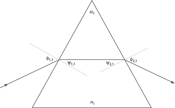
FIGURE 2.19 Single prism depicting refraction at minimum deviation.

ϕ_{1} + ϕ_{2} = ॉ + α (2.58)

$ϕ_{1} + ϕ_{2} = ॉ + α (2.58)$

ψ_{1} + ψ_{2} = α (2.59)

$ψ_{1} + ψ_{2} = α (2.59)$

\sin (ϕ_{1} = n \sin ψ_{1} (2.60)

$\sin (ϕ_{1} = n \sin ψ_{1} (2.60)$

\sin ϕ_{2} = n \sin ψ_{2} (2.61)

$\sin ϕ_{2} = n \sin ψ_{2} (2.61)$

where:

ϕ₁ and ϕ₂ are the angles of incidence and emergence

ψ₁ and ψ₂ are the corresponding angles of refraction

α is the apex angle

ε is the angle of deviation

n is the index of refraction of the prism

Differentiating Equation 2.59 with respect to n, we obtain the identity

\frac{d ψ_{1}}{d n} = - \frac{d ψ_{2}}{d n} (2.62)

$\frac{d ψ_{1}}{d n} = - \frac{d ψ_{2}}{d n} (2.62)$

and differentiating Equations 2.60 and 2.61, we obtain

\frac{d ϕ_{2}}{d n} = \frac{\sin ψ_{2}}{\cos (ϕ_{2}} + (\frac{\cos ψ_{2}}{\cos (ϕ_{2}}) \tan ψ_{1} (2.63)

$\frac{d ϕ_{2}}{d n} = \frac{\sin ψ_{2}}{\cos (ϕ_{2}} + (\frac{\cos ψ_{2}}{\cos (ϕ_{2}}) \tan ψ_{1} (2.63)$

which is the result given by Born and Wolf (1999). The use of the identity

\frac{d (ϕ_{2}}{d λ} = (\frac{d (ϕ_{2}}{d n}) (\frac{d n}{d λ}) (2.64)

$\frac{d (ϕ_{2}}{d λ} = (\frac{d (ϕ_{2}}{d n}) (\frac{d n}{d λ}) (2.64)$

provides the dispersion for a single prism (Duarte 1990):

\frac{d ϕ_{2}}{d λ} = [\frac{\sin ψ_{2}}{\cos (ϕ_{2}} + (\frac{\cos ψ_{2}}{\cos (ϕ_{2}}) \tan ψ_{1}] \frac{d n}{d λ} (2.65)

$\frac{d ϕ_{2}}{d λ} = [\frac{\sin ψ_{2}}{\cos (ϕ_{2}} + (\frac{\cos ψ_{2}}{\cos (ϕ_{2}}) \tan ψ_{1}] \frac{d n}{d λ} (2.65)$

which for orthogonal beam exit, that is, ϕ₂ ≈ ψ₂ ≈ 0, becomes

\frac{d ϕ_{2}}{d λ} \approx \tan ψ_{1} \frac{d n}{d λ} (2.66)

$\frac{d ϕ_{2}}{d λ} \approx \tan ψ_{1} \frac{d n}{d λ} (2.66)$

The generalized multiple-prism dispersion, for both positive and negative diffraction, is considered in detail in Chapter 4.

2.8 Dirac and the Laser

In his seminal discussion on interference, in 1930, Dirac introduced the concept of interference as a one-photon phenomenon (Dirac 1978). Explicitly, he stated, “Each photon then interferes only with itself. Interference between two different photons never occurs” (p. 9). This concept is central to explain the physics of the N-slit interferometer since it is a single photon that illuminates the whole array of N slits, or grating, simultaneously. In the case of a monochromatic laser beam or an ensemble of indistinguishable photons, or indistinguishable quanta, all the indistinguishable photons illuminate the array of N slits, or grating, simultaneously. In the past, this concept has been the source of some controversy due to a misunderstanding of the Dirac interpretation, which implies that indistinguishable photons, regardless of source of origin, are the same photons.

As explained in Chapter 11, interference a là Dirac, utilizing indistinguishable photons, via

| 〈 x | s 〉 |^{2} = \sum_{j = 1}^{N} Ψ (r_{j})^{2} + 2 \sum_{j = 1}^{N} Ψ (r_{j}) [\sum_{m = j + 1}^{N} Ψ (r_{m}) \cos (Ω_{m} - Ω_{j})]

$| 〈 x | s 〉 |^{2} = \sum_{j = 1}^{N} Ψ (r_{j})^{2} + 2 \sum_{j = 1}^{N} Ψ (r_{j}) [\sum_{m = j + 1}^{N} Ψ (r_{m}) \cos (Ω_{m} - Ω_{j})]$

yields spatially sharp, well-defined interferograms with a high degree of visibility near unity. Due to the integrated and cumulative nature of the detection process (Duarte 2004, 2008), interferograms from semicoherent sources produce interferograms with broad features, lower spatial definition, and decreased visibility (see Figure 11.11). At the other extreme, plainly distinguishable photons, or photons of distinct different wavelengths (such as a blue photon and a red photon), do not interfere with each other.

The Dirac discussion on the interference of photons goes even further. It begins with reference to a beam of roughly monochromatic light, and then prior to his dictum on interference, he wrote about a beam of light having a large number of photons. It is this beam of light that in his discussion is divided into two components and is subsequently made to interference. In present terms, this is no different than the description of interference due to the interaction of a high-power narrow-linewidth laser beam with a two-beam interferometer (Duarte 1998). In other words, in 1930 Dirac provided perhaps the earliest physical description of a laser beam, laser interference, and hence, laser optics.

Problems

2.1 Show that substitution of Equations 2.5 and 2.6 into Equation 2.3 leads to Equation 2.7.

2.2 Show that Equation 2.12 can be expressed as Equation 2.13.

2.3 From the geometry of Figure 2.7, derive Equations 2.22 through 2.24.

2.4 Write an equation for |〈x | s〉|² in the case relevant to Figure 2.12, that is, an N-slit grating illuminated by a wide single slit. Assume that the single wide slit can be represented by an array of N subslits.

2.5 Show that, for orthogonal beam exit, Equation 2.65 reduces to Equation 2.66.

..................Content has been hidden....................

You can't read the all page of ebook, please click here login for view all page.

Table of Contents for
Chapter 2 Dirac Optics

2

Dirac Optics

2.1 Introduction

2.2 Dirac’s Notation in Optics

2.3 Interference

2.3.1 Example

2.3.2 Geometry of The N-Slit Interferometer

2.3.3 N-Slit Interferometer Experiment

2.4 Generalized Diffraction

2.4.1 Positive Diffraction

2.5 Positive and Negative Refraction

2.6 Reflection

2.7 The Cavity Linewidth Equation

2.7.1 Introduction to Angular Dispersion

2.8 Dirac and the Laser

Problems

Table of Contents for Chapter 2 Dirac Optics

Create new playlist

Sign In

Sign Up

Table of Contents for
Chapter 2 Dirac Optics