
10
The N-Slit Laser Interferometer Optical Architecture and Applications
10.1 Introduction
In this chapter, attention is given to one particular optical architecture that integrates several concepts introduced in Chapters 2, 4 and 6 and has various applications in imaging and metrology. That particular optical architecture is that of the N-slit laser interferometer (NSLI). Depending on the application, the NSLI can be configured with a narrow-linewidth tunable laser or a narrow-linewidth fixed-frequency laser.
10.2 Optical Architecture of the NSLI
The NSLI is illustrated in Figure 10.1. In its basic configuration, this interferometer requires the illumination from a laser emitting in a single transverse mode (TEM00) with narrow-linewidth characteristics, which ideally should be confined to a single longitudinal mode (SLM). The beam is magnified by a two-dimensional transmission telescope, such as a Galilean telescope, and then propagates through an optional convex lens, which is necessary for microscopic and microdensitometry applications. Transmission through a telescope–convex lens combination yields a very tightly focused beam with an excellent depth of focus. Propagation of this beam, through a multiple-prism beam expander, maintains the focusing in the plane transverse to the plane of propagation and expands the beam in the plane of propagation. The result is an extremely elongated near-Gaussian beam typically 25 μm in height and 25,000 μm in width (see Figure 10.2). Note that this telescope–lens–multiple-prism configuration can easily yield additional beam expansion; for instance, Duarte (1987) reported on extremely elongated Gaussian beams 20 μm in height and 60,000 μm in width, that is, a spatial height-to-width ratio of 1:3000.
Albeit we refer here to these beam profiles as extremely elongated Gaussian beams, it should also be mentioned that particularly in the fields of microscopy, and nanoscopy, this type of illumination is also known as thin light-sheet illumination and selective plane illumination.
An alternative configuration includes the deployment of the focusing convex lens post multiple-prism expander. Also, straightforward interferometric configurations do not require the convex lens as part of the architecture. However, for the sake of completeness in the following analysis, the convex lens is included.
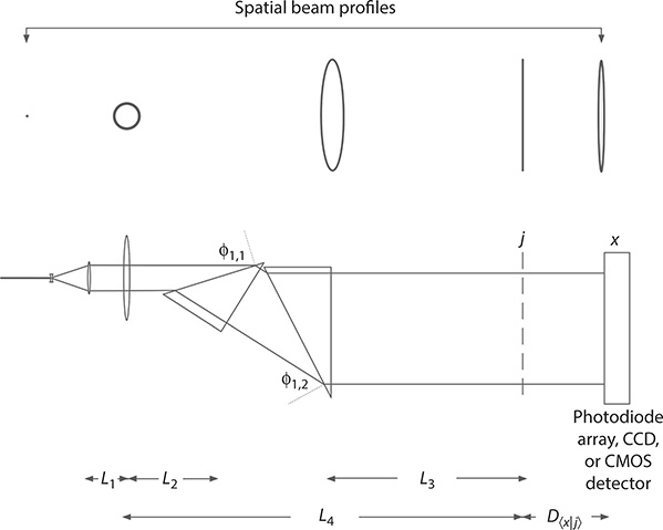
FIGURE 10.1 NSLI depicting the Galilean telescope, the focusing lens, the multiple-prism beam expander, the position of the N-slit array (j), or transmission surface of interest, and the interferometric plane (x). The intra-interferometric distance from j to x is D〈x | j〉. A depiction of approximate beam profiles, at various propagation stages, is included on top. This drawing is not to scale.
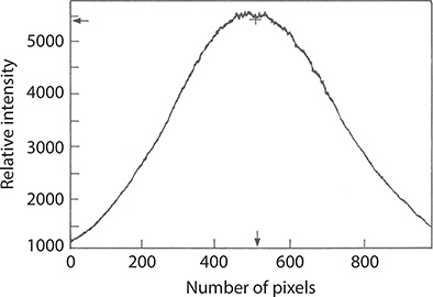
FIGURE 10.2 Intensity profile of an extremely elongated, approximately 1:1000 (height: width), near-Gaussian laser beam.
At this stage, it should be noted that the one-dimensional beam expansion parallel to the plane of propagation (or plane of incidence) is provided by a multiple-prism beam expander (Duarte 1987, 1991, 1993b) since this form of beam expansion does not introduce further focusing variables. Further, the multiple-prism beam expander can be designed to yield zero dispersion at a chosen wavelength of design (Duarte and Piper 1982; Duarte 1985) as described in Chapter 4.
As illustrated in Figure 10.1, the expanded laser beam illuminates the N-slit array at j where N sub-beams are created and proceed to propagate toward the detection screen at x, which is configured by a digital detector. Following some spatial displacement after j, the N sub-beams, due to divergence mandated by the uncertainty principle, begin to undergo interference since all these beams are composed of undistinguishable photons. The pattern of interference is recorded by the detector at x at the distance D〈x | j〉 from the N-slit array. Note that although the detector of choice is a digital detector, such as a photodiode array, charge-coupled device (CCD), or complementary metal–oxide–semiconductor (CMOS) array, photographic detection can also be used. If detection is provided by a linear array of microscopic detectors, then, as explained in Chapter 2, the spatial distribution of the interference signal can be described by
which can be expressed as (Duarte and Paine 1989; Duarte 1991)
Interference in two dimensions is described by (Duarte 1995)
Equation 10.2 has been successfully applied to characterize the interference resulting from the interaction of expanded narrow-linewidth laser beams slit arrays of various dimensions and N in the range of 2 ≤N ≤ 2000 (see, e.g., Duarte 1993b, 1995).
10.2.1 Beam Propagation in the N SLI
The first stage of design is to optimize the transmission of the laser beam to the N-slit array. Although the telescope–convex lens system is polarization neutral, the multiple-prism beam expander has a strong transmission preference for radiation polarized parallel to the plane of propagation (see Chapter 5). The first step consists in matching the polarization of the laser to the polarization preference of the multiple-prism beam expander. For the mth prism, this transmission can be characterized using the expression
for the incidence surfaces and
for the exit surfaces. The equations for the respective losses are given in Chapter 5 and are
and
where:
ℛ1,m and ℛ2,m are given by
Note that given the inherent high intensity of laser sources, for most applications the use of antireflection coatings at the optics is not necessary.
The ray transfer matrix at the plane of propagation is given by (Duarte 1993a)
where the following quantities correspond to the multiple-prism beam expander:
and
where:
Lm is the distance separating the prisms
lm is the path length at the mth prism
Also, Mt and Bt correspond to the A and B terms of the transfer matrix for the Galilean telescope given in Chapter 6 and
In the above equations, L1 is the distance between the telescope and the lens, L2 is the distance between the lens and the multiple-prism beam expander, and L3 is the distance between the multiple-prism beam expander and the N-slit array (see Figure 10.1).
For the vertical component, the ray transfer matrix is given by
where:
L4 is the distance between the lens and the N-slit array
In the absence of the convex lens following the two-dimensional telescope, Equations 10.9 and 10.15 reduce to
and
The width of the Gaussian beam can be calculated using the expression given by Turunen (1986)
where:
the A and B terms are given by Equations 10.9 and 10.15, if using a convex lens, or by Equations 10.16 and 10.17 in the absence of a convex lens
is the Rayleigh length
The focused extremely elongated near-Gaussian coherent illumination is used in nanoscopic, microscopic, and microdensitometry applications (Duarte 1993a, 1993b) requiring illumination of N-slit arrays with transverse nanoscopic or microscopic dimensions. The unfocused elongated near-Gaussian illumination is used in conventional interferometric measurements (Duarte 2002, 2005; Duarte et al. 2010, 2011, 2013).
10.2.1.1 Example
In a propagation example discussed by Duarte (1995), λ = 632.82 nm, w0 = 250 μm, M = 5.75, Mt = 20, f = 30 cm, and the elongated near-Gaussian beam becomes 53.4 mm wide by 32.26 μm high at the focal plane. Notice that the parameters in Equation 10.14 are chosen so that condition ζ ≈f is met and the width of the beam is dominated by the product MMt. Appropriate selection of the distance from the lens to the focal plane also makes L4 ≈ f so that the vertical dimension of the beam, determined by the A and B terms of Equation 10.15, becomes very small. The intensity profile of an expanded near-Gaussian beam with a spatial height-to-width ratio of approximately 1:1000 is shown in Figure 10.2. Removal of the convex lens yields a near-Gaussian beam approximately 53.4 mm wide by 10 mm high.
10.3 An Interferometric Computer
Interferograms recorded with the NSLI have been compared for numerous geometrical and wavelength parameters with interferograms calculated via Equation 10.1 or 10.2. One such case is reproduced in Figure 10.3. In this regard, it should be mentioned that good agreement, between theory and experiment, exists from the near to the far field. Slight differences, especially at the baseline, are due to thermal noise in the digital detector that is used at room temperature. The interferometric calculations, using Equations 10.1 through 10.3, require the following input information:
Slit dimensions, w
Standard deviation of the slit dimensions, Δw
Interslit dimensions
Standard deviation of interslit dimensions
Wavelength, λ
N-slit array, or grating, screen distance, D〈x | j〉
Number of slits, N
The program also gives options for the illumination profile and allows for multiple-stage calculations. That is, it allows for the propagation through several sequential N-slit arrays prior to arrival at x as considered in Chapter 2.
An interesting aspect of comparisons, between theory and experiment, is that for a given wavelength, a set of slit dimensions, and a distance from j to x, calculations in a conventional universal computer take longer as the number of slits N increases. In fact, the computational time t(N) behaves in a nonlinear fashion as N increases. This is clearly illustrated in Figure 10.4, where t = 0.96 s for N = 2 and t = 3111.2s for N = 1500 (Duarte 1996). By contrast, all of these calculations can be performed in the NSLI at a constant time of ~30 ms, which is a time mainly imposed by the integration time of the digital detector.
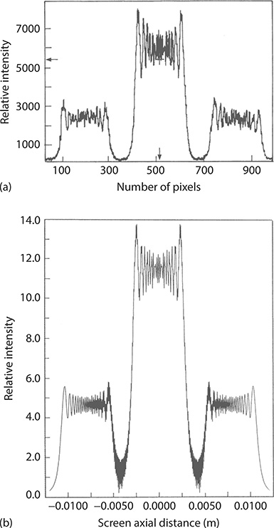
FIGURE 10.3 Measured interferogram (a) and calculated interferogram (b). Slits are 30 μm wide, separated by 30 μm, and N = 100. The intra-interferometric distance is D〈x | j〉 75 cm and λ = 632.82 nm. This calculation assumes uniform illumination (see Chapter 2). (Reprinted from Opt. Commun., 103, Duarte, F.J., On a generalized interference equation and interferometric measurements, 8–14, Copyright 1993b, with permission from Elsevier.)
In this regard, following the criteria outlined by Deutsch (1992), the NSLI can be classified as a physical, or interferometric, computer that can perform certain specific computations at times orders of magnitude below the computational time required by a universal computer. Among the computations that the interferometric computer can perform are as follows:
N-slit array interference calculations
Near- or far-field diffraction calculations
Beam divergence calculations
Wavelength calculations
For these tasks, the interferometric computer based on the NSLI outperforms, by orders of magnitude, universal computers. Hence, it can be classified as a very fast, albeit limited in scope, optical computer. The advantage of the universal computer remains its versatility and better signal-to-noise ratio. Also, in the universal computer, there is access to intermediate results at all stages of the computation. This is not allowed in the NSLI where access is strictly limited to the input stage and the final stage of the computation. Attempts to acquire information about the intermediate stages of the computation destroy the final answer.
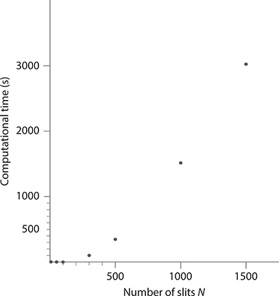
FIGURE 10.4 Computational time, in a universal computer, as a function of the number of slits. For these calculations, the slit width is 30 μm, the interslit width 30 μm, the j-to-x distance is D〈x | j〉 75 cm, and λ = 632.28 nm. (Data from Duarte, F.J., Proceedings of the International Conference on Lasers ‘95, STS Press, McLean, VA, 1996.)
See Duarte (2014) for a discussion of quantum computing using qubits.
10.4 Secure Interferometric Communications in Free Space
Optical signals in free space have been used in the field of communications since ancient times. An example to optical communications in a modern context is the use of Morse code. More recent interest in this field has produced a variety of laser-based optical architectures and approaches (Yu and Gregory 1996; Boffi et al. 2000; Willebrand and Ghuman 2001). Prevalent among the secure approaches offering secure communications is quantum cryptography (Bennett and Brassard 1984; Duarte 2014). Here, an alternative approach to secure optical communications in free space, based on interferometric communications, is introduced and described.
For a given set of geometrical parameters and wavelength, the NSLI yields a unique interferogram that can be accurately matched to its theoretical counterpart given by
which was introduced in detail in Chapter 2. This feature can be utilized in the field of optical communications to perform secure communications in free space. The optical architecture of the NSLI used for this application is as described earlier with one modification that the distance from the N-slit array (j) to the digital detector (x) can be very large and allowances are made for a beam splitter, representing a possible intruder, to be inserted in the optical path between j and x, that is, D〈x | j〉 . This modified, long-path length, NSLI is depicted in Figure 10.5. Again, the critical parameters determining the interferometric distribution are the narrow-linewidth laser wavelength λ, the slit width, the number of slits, and the intra-interferometric distance from the N-slit array (positioned at j) to the interference plane (positioned at x), which is denoted by the quantity D〈x | j〉 in Figure 10.5.
The principle of operation is extraordinarily simple: any optical distortion introduced in the intra-interferometric optical path D〈x | j〉 alters the predetermined inter-ferogram recorded at x. Thus, the receiver at x immediately detects the presence of an intruder or eavesdropper in the optical path of communications. This means that interferometric communications provide a simple alternative to secure communications in free space. The method is particularly suited to provide secure communications in outer space.
As described by Duarte (2002), secure interferometric communications using the NSLI relies on an interferometric alphabet where an alphabetic character such as an a is related to a specific interferogram. Four possible interferometric characters corresponding to a, b, c, and z are shown in Figure 10.6. Here, the letter a is represented by two slits (N = 2), the letter b by three slits (N = 3), the letter c by four slits (N = 4), and so on. In these calculations, the slits are 50 μm wide and are separated by 50 μm at λ = 632.82 nm. Certainly, there is a limitless choice of alphabetic characters.

FIGURE 10.5 Very large NSLI configured without the focusing lens. In this class of interferometer, the intra-interferometric path is in the 7 ≤ D〈x | j〉 ≤ 527 m range, although larger configurations are possible. In these NSLIs, the TEM00 beam from the He–Ne laser is transmitted via a spatial filter. (Reproduced from Duarte, F.J., et al., J. Opt., 12, 015705, 2010. With permission from the Institute of Physics.)
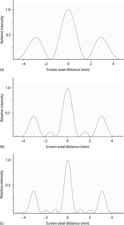
FIGURE 10.6 Interferometric alphabet: (a) a (N = 2); (b) b (N = 3); (c) c (N = 4).
Transmission integrity is demonstrated in Figure 10.7 for the case of the interferometric character a (N = 2). To this effect, an optically smooth surface with an average thickness of ~150 μm is introduced, at an angle, in the optical path to cause a reflection of the charactera. It should be noted that insertion of the beam splitter normal to the optical axis produces no measurable spatial optical distortions except a decrease in the intensity of ~8%.

FIGURE 10.6 (d)z (N = 26). For these calculations, the slits are 50 μm, separated by 50 μm, D〈x | j〉 50 cm, and λ = 632.82 nm.
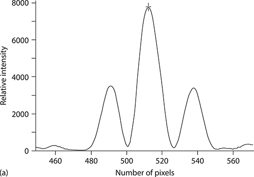
FIGURE 10.7 Interception sequence for the interferometric character a (N = 2) the slits are 50 μm, separated by 50 μm, D〈x | j〉 10 cm, and λ = 632.82 nm. (a) Original interferometric character. (b–d) Show the distortion sequence of the interferometric character due to the insertion of a thin beam splitter into the optical path. (e) Interferometric character a showing slight distortion and displacement due to the stationary beam splitter. (Reprinted from Opt. Commun., 205, Duarte, F.J., Secure interferometric equations in free space, 313–319, Copyright 2002, with permission from Elsevier.)
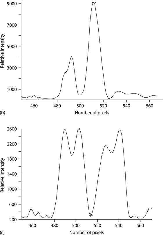
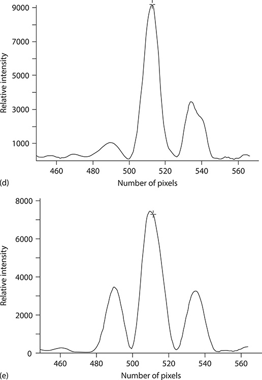
The angle of incidence of the interferometric character on the beam splitter was selected to be close to the Brewster angle of incidence to reduce transmission losses while still being able to reflect a measurable fraction of the signal. In the sequence of measurements, Figure 10.7a shows the original undistorted character a. The severe distortions depicted in Figure 10.7b–d show the effect of introducing the thin beam splitter in the optical path. Figure 10.7e depicts the intercepted interferometric character a. Although the severe distortions are no longer present, close scrutiny of the interferogram reveals a decrease by ~3.7% in the intensity of the signal relative to the original character shown in Figure 10.7a. The intercepted signal is also displaced by approximately 50 μm, in the frame of reference of the detector, due to the refraction induced at the beam splitter. In addition, there is a slight obliqueness in the intensity distribution as determined from the secondary maxima. Hence, in comparison with the original interferometric character or a theoretically generated character, it can be concluded that the integrity of the intercepted character a has been distinctly compromised.
Although the measurements considered above were performed over short propagation path lengths in the laboratory, of 0.1 and 1 m, Duarte (2002) also discussed propagation over larger distances. Using interferometric calculations, via Equation 10.2 or 10.3, it can be shown that communications in free space can proceed over long path lengths using visible wavelengths and a detector comprising a few tiled photodiode arrays. One specific example involves the generation of the interferometric character a using two 1 mm slits separated by 1 mm. For λ = 632.82 nm, this arrangement produces an interferometric distribution bound within 10 cm for a propagation path length of 100 m. The interferometric character z is produced by an array of N = 26 slits of 1 mm, separated by 1 mm. For λ = 632.82 nm, this arrangement produces an interferometric distribution bound within 14 cm for a propagation path length of 100 m. This can be accomplished using two linear photodiode arrays (each 72 mm long) tiled together. If the dimensions of the slits are increased to 3 mm, at λ = 441.16 nm, interferometric characters could be propagated over distances of 1000 m using four such tiled photodiode arrays (Duarte 2002).
10.4.1 Very Large N Slis for Secure Interferometric Communications in Free Space
The examples considered up to now assume a propagation intra-interferometric path D〈x | j〉 characterized by a single homogeneous propagation medium, such homogeneous air or vacuum, between j and x.
Free-space communications in terrestrial environments of interferometric characters would need to account for the inherent atmospheric turbulence present in such surroundings. This would certainly detract from the simplicity of the method. This could still be accomplished, noting that atmospheric distortions are stochastic in nature compared to systematic distortions introduced by optical interception.
D〈x | j〉 has been extended experimentally to the meter range (Duarte 2005), to 35 m (Duarte et al. 2010), and to 527 m (Duarte et al. 2011).
The c interferometric character (N = 4), generated with 570 μm-wide slits separated by 570 μm, using λ = 632.82 nm, at D〈x | j〉 7.235 m is shown in Figure 10.8. Interception of this interferometric character by a high-optical-quality ultrathin beam splitter at Brewster’s angle produces the collapse of the interferogram as illustrated in Figure 10.9. Interception of the interferometric character by mild air turbulence, generated by a heat source, yields mild distortions of the c interferometric character as illustrated in Figure 10.10.
The c interferometric character (N = 4), generated with 1000 μm-wide slits separated by 1000 μm, using λ = 632.82 nm, at D〈x | j〉 35 m in open air at T ≈ 30°C is shown in Figure 10.11. Visible here is a very slight distortion of the interferometric character due to very mild atmospheric turbulence. This led to the observation that the NSLI is applicable as an effective detector of clear air turbulence and could be deployed, using infrared lasers, at the thresholds of aviation runways to alert pilots of any possible detrimental turbulence (Duarte et al. 2010).

FIGURE 10.8 The interferometric character c (N = 4). Here, the slits are 570 μm, separated by 570 μm, D〈x | j〉 = 7.235 m, and λ = 632.82 nm. (Reproduced from Duarte, F.J., J. Opt. A: Pure Appl. Opt., 7, 73–75, 2005. With permission from the Institute of Physics.)
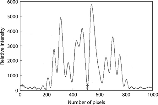
FIGURE 10.9 The interferometric character c (N = 4), as described in Figure 10.8, destroyed by optical interception. See text for further details. (Reproduced from Duarte, F.J., J. Opt. A: Pure Appl. Opt., 7, 73–75, 2005. With permission from the Institute of Physics.)
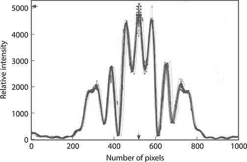
FIGURE 10.10 The interferometric character c (N = 4), as described in Figure 10.8, distorted due to turbulence generated by a thermal source. See text for further details. (Reproduced from Duarte, F.J., Tunable Laser Applications, CRC Press, New York, 2009. With permission from Taylor & Francis.)
Experiments at D〈x | j〉 527 m also led to the discovery that the interferometric characters could be intercepted and modified in a controlled nondestructive, or nondemolition, manner using transparent spider silk web fibers (Duarte et al. 2011). Indeed, accurate knowledge of the position of the fiber relative to the propagating interferometric character leads to an accurate prediction of the interferometric character showing a superimposed diffraction signature created by the interaction of the spider web fiber (with a diameter in the 25–30 μm range) with the N-slit interferogram.
For the b interferometric character (N = 3) generated with 570 μm-wide slits separated by 570 μm, using λ = 632.82 nm, at D〈x | j〉 = 7.235 the control interferogram is shown in Figure 10.12. Inserting the spider web fiber 15 cm from the x plane (or CCD detector) at D〈x | j〉 = 7.235 - 0.150 yields a measured interferogram as illustrated in Figure 10.13. Representation of the spider web fiber as two wide slits separated by 25 μm while using
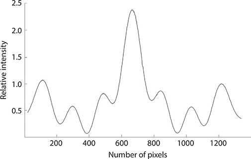
FIGURE 10.11 The interferometric character c (N = 4) showing a slight unevenness due to incipient atmospheric turbulence. Here, the slits are 1000 μm, separated by 1000 μm, D〈x | j〉 35 m, and λ = 632.82 nm. (Reproduced from Duarte, F.J., et al., J. Opt., 12, 015705, 2010. With permission from the Institute of Physics.)
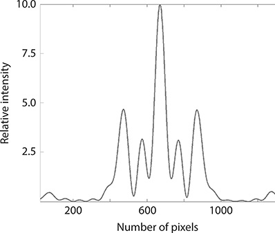
FIGURE 10.12 The interferometric character b (N = 3) used as a control. Here, the slits are 570 μm, separated by 570 μm, D〈x | j〉 = 7.235 m, and λ = 632.82 nm. (Reproduced from Duarte, F.J., et al., J. Mod. Opt., 60, 136–140, 2013. With permission from Taylor & Francis.)

FIGURE 10.13 The interferometric character b (N = 3) intercepted by a spider web silk fiber positioned at D〈x | j〉 = 7.235 − 0.150 m. The slits are 570 μm, separated by 570 μm; the interferogram is recorded at D〈x | j〉 = 7.235 m and λ = 632.82 nm. (Reproduced from Duarte, F.J., et al., J. Mod. Opt., 60, 136–140, 2013. With permission from Taylor & Francis.)
in a cascade approach (Duarte 1993b) where the predicted interferogram at D〈x | j〉 = 7.235 − 0.150 m becomes the input distribution at the new array yields the calculated interferogram illustrated in Figure 10.14, which agrees closely with the measured interferogram of Figure 10.13 (Duarte et al. 2013; Duarte 2014). These results illustrate that albeit it is possible to interact nondestructively with the propagating interferogram, the presence of the interception is still detected. More subtle, harder to detect nondemolition interactions are discussed by Duarte et al. (2013) and Duarte (2014).

FIGURE 10.14 Theoretical interferometric character b (N = 3) assuming interception by a spider web silk fiber positioned at D〈x | j〉 = 7.235 − 0.150 m (see text). The slits are 570 μm, separated by 570 μm; the interferometric plane is positioned at D〈x | j〉 = 7.235 m and λ = 632.82 nm. (Reproduced from Duarte, F.J., et al., J. Mod. Opt., 60, 136–140, 2013. With permission from Taylor & Francis.)
One modification applicable to these large and very large NSLIs would be the introduction of a distortionless high-fidelity beam expander, such as an optimized multiple-prism beam expander. In Chapter 4, it was shown that these expanders can easily provide beam magnification factors of M ≈ 100. Deployment of such multiple-prism beam expander next to the slit array would reduce the beam divergence significantly, thus reducing the requirements on the dimensions of the digital detectors. From a technological viewpoint, it is important to emphasize the use of TEM00 lasers with narrow-linewidth, preferably SLM, emission since that characteristic is essential in providing well-defined sharp high-visibility interferometric characters close to their theoretical counterparts. The characters could be changed in real time either by using a tunable laser or by incorporating precision variable slit arrays. The use of narrow band-pass filters could allow transmission during daylight.
Quantum cryptography provides secure optical communications guaranteed by the quantum entanglement of polarizations (Pryce and Ward 1947; Ward 1949) and has been shown to be applicable over distances of tens of kilometers [see Duarte (2014) for a recent review]. Interferometric communications using the NSLI provides security using the principle of interference. As outlined in Chapter 3, the uncertainty principle itself can be formulated from interferometric arguments. Advantages of free-space communications using interferometric characters include a very simple optical architecture and the use of relatively high-power narrow-linewidth SLM lasers, although the method also applies to single-photon emission.
As a final point of interest, it can be shown that the quantum entanglement of polarizations also has an interferometric origin (Duarte 2013, 2014) as outlined in Chapter 3.
10.5 Applications of the NSLI
In this section, various applications of the NSLI are described. First, it is discussed as a digital laser microscope (DLM) and as a tool to perform light modulation measurements in imaging. Next, its application in secure optical communications is considered. The section concludes with a discussion on wavelength and temporal measurements.
10.5.1 Digital Laser Micromeasurements
Micromeasurements are widely applied in the field of imaging. One such class of measurements, called microdentitometry, was described by Dainty and Shaw (1974). In a traditional microdensitometer, a beam of light, with a diameter typically in the 10–50 μm range, is used to illuminate a transmission surface. The ratio of the transmitted intensity (It), through the surface, over the incident intensity (Ii) is a measure of the transmission and the density is defined as (Dainty and Shaw 1974)
Thousands of measurements over the surface yield an average density and a standard deviation. The standard deviation is a measure of the so-called granularity, or σ and is a parameter widely used to evaluate the microdensity characteristics of transmission imaging materials such as photographic films. Typically, the optical density of photographic films varies in the 0.1 ≤D ≤ 3.0 range. A low granularity value, indicating a fine film, would be in the 0.001 ≤ σ ≤ 0.005 range. Traditional high-speed microdensitometers using incoherent illumination sources face various challenges, including adverse signal-to-noise ratios, to determine microdensity variations in very fine imaging surfaces and very short depths of focus.
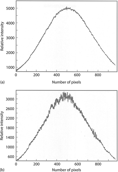
FIGURE 10.15 Transmission signal showing no interference from an optical homogeneous imaging surface (a) and interferogram from an imaging surface including relatively fine particles (b).
The use of the NSLI as a DLM was introduced by Duarte (1993b, 1995). In a DLM, an extremely elongated near-Gaussian beam illuminates, at its focal point, the width of the imaging surface of interest. The interaction of the expanded illumination beam with the imaging surface at j yields an interference pattern at x. In this regard, the imaging surface at j can be considered as a regular, or an irregular, transmission grating, and the interference pattern at x is unique to that imaging surface. If the smooth expanded illumination distribution, illustrated in Figure 10.15a, is defined as Ii(x, λ), and the transmitted interferometric signal as It(x, λ), then the optical density can be defined as
This equation provides the macrodensity of the surface under illumination. The microdensity is obtained by exploiting the spatial dependence of the transmitted interferogram in conjunction with the spatial discrimination available from the digital detector. In order to illustrate this mode of operation, consider a unilayer film of very fine grains. The slits of very small dimensions cause, according to the uncertainty principle, a high divergence, which implies that the interferometric pattern at x is characterized by fine features of moderate modulation. By contrast, a unilayer film of coarser grains, or slits of larger dimensions, causes less divergence so that the interference pattern at x is characterized by coarser features and larger modulation. This comparison is illustrated in Figure 10.15.
The average microdensity, at a given wavelength, is obtained from
The standard deviation of this quantity is a measure of the granularity, or σ, of the imaging surface. The number N is determined by the number of pixels in the digital detector, which is typically 1024 or 2048. The size of the sampling depends on the dimensions of the pixels that vary from a few micrometers to 25 μm.
Detailed cross-over measurements between traditional microdensitometers, with incoherent illumination, and the DLM have yielded very good agreement of macrodensities and similar behavior in σ as a function of D. Absolute values of σ in the DLM tend to be higher than the values determined with traditional means. One essential advantage of the DLM is that from interferograms such as those displayed in Figure 10.15 it is possible to determine the average size of the slits causing the interference. Further characteristics that make DLMs very attractive are as follows:
A dynamic range approaching 109
A signal-to-noise ratiô107
A depth of focus greater than 1 mm
Simultaneous collection of a large number of data points
From an imaging perspective, it should be mentioned that the mathematical form of Equation 10.3 is similar to the equation of power spectrum, which is widely applied in traditional studies of microdensitometry.
A simple modification of the optical architecture transforms the DLM from a transmission mode to a reflection mode as illustrated in Figure 10.16. The same physics applies. This configuration is useful to determine surface characteristics of imaging surfaces.
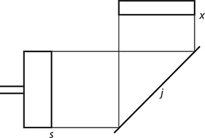
FIGURE 10.16 NSLI configured in the reflection mode.
10.5.2 Light Modulation Measurements
Modulation transfer measurements are extensively used in imaging to determine the spatial resolution of transmission gratings configured by coatings of various materials. In principle, the technique is quite simple and consists in coating regular N-slit gratings, with a given material, for a series of spatial frequencies. Then the near-field modulation of the light transmitted via these gratings is recorded as a function of spatial frequency. In transmission gratings comprising imaging materials of a crystalline nature, the spatial resolution decreases as the spatial frequency increases. This is manifested in a deterioration of the light modulation as the spatial frequency increases.
The NSLI can be applied in a straightforward manner to quantify the modulation of light, by a given transmission grating, by configuring the interferometer with a fairly short j-to-x distance. This is demonstrated in Figure 10.17. Here, a grating made from a metallic coating with slits 100 μm wide, separated by 100 μm, and N = 23 is illuminated with an expanded near-Gaussian beam at λ = 632.82 nm. The j-to-x distance, that is, D〈x | j〉 , is 1.5 cm. Note that, at this grating-to-detector distance, for the slit dimensions given, interference is rather weak and does not dominate the modulation of the signal. A theoretical version of the signal is given in Figure 10.17b.
Comparison between theory and experiment shows that the depth of modulation even for a metallic coating, ~90% in this case, is less than the theoretical modulation. Transmission gratings made from photographic coatings can show a significant deterioration in modulation for spatial frequencies beyond ~40 lines/mm.
10.5.3 Wavelength Meter and Broadband Interferograms
Generalized N-slit interference equations, such as Equations 10.2 and 10.3, are inherently wavelength dependent, since the interference term is a function of wavelength as explained in Chapter 2. Thus, it is straightforward to predict that, for a fixed set of geometrical parameters, the measured interferogram depends uniquely on the wavelength of the laser. This feature can be applied to use the NSLI as a wavelength meter as explained in detail in Chapter 11.
Albeit emphasis has been made up to now on the desirability of using narrow-linewidth lasers, in conjunction with the NSLI, the scope of the measurements can also be extended to include broadband emission. For broadband emission sources, the measured interferogram represents a cumulative interferogram, resulting from a series of individual wavelengths, as illustrated in Figure 10.18. This concept is central to this measurement approach and it is based on Dirac’s dictum on interference (Dirac 1978). That is, interference occurs between undistinguishable photons only. In other words, blue photons do not interfere with green or red photons. Hence, an interferogram with broad features, as illustrated in Figure 10.18, is a cumulative signal integrated by a series of individual interferograms arising from a series of different wavelengths (see Chapter 11). Once the central wavelength of emission of the broadband interferometer is determined, using a standard spectrometer or suitable wavelength meter, a theoretical cumulative interferogram can be constructed to match the measured signal and determine its bandwidth.

FIGURE 10.17 Near-field modulation signal in a weak interferometric domain arising from the interaction of laser illumination, at λ = 632.82 nm, and a grating composed of N = 23 slits 100 μm wide separated by 100 μm. The intra-interferometric distance is D〈x | j〉 = 15. cm. Measured modulation signal (a) and calculated signal (b). Each pixel is 25 μm wide. (Reprinted from Opt. Commun., 103, Duarte, F.J., On a generalized interference equation and interferometric measurements, 8–14, Copyright 1993b, with permission from Elsevier.)
In principle, for broadband ultrashort pulsed lasers, once the bandwidth of the emission is determined, an approximate estimate of the temporal pulse duration is possible using the time–frequency uncertainty relation ΔνΔt ≈ 1. This simple concept is only applicable to ultrashort pulse lasers emitting pulses and spectral distributions obeying the time–frequency uncertainty limit.
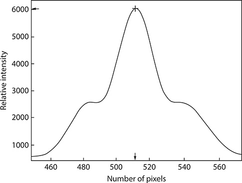
FIGURE 10.18 Measured double-slit interferogram generated using a broadband visible light source. The slits are 50 μm wide separated by 50 μm and the intra-interferometric distance is D〈x | j〉 10 cm.
10.5.4 Imaging Laser Printers
Traditional sensitometry and sensitometers are described by Altman (1977). In essence, a sensitometer is an instrument that illuminates an unexposed imaging material to produce a series of exposures at various light intensity levels. A laser sensitometer uses stable lasers yielding TEM00 beams and various optical techniques to print a scale of exposures that can then be optically characterized to determine the sensitivity of the imaging material. In this section, the optical architecture of a multiple-laser sensitometer, or multiple-laser printer, is described.
Laser sensitometers work on the principle of exposing a line by displacing a focused near-Gaussian beam with a beam waist in the 60 ≤w ≤ 100 μm range. This line is exposed on the imaging material that is deployed at a plane perpendicular to the optical axis and to the plane of propagation. The imaging medium is displaced, orthogonal to the plane of propagation, at a velocity allowing for an overlap (usually 50%) of the near-Gaussian beam. The movement of the laser beam provides the temporal component of the exposure. Once an exposure of certain dimensions is produced, usually 10 mm in width, the intensity of the laser beam is adjusted, using electro-optical means, and a new series of line exposures is produced. Eventually a scale of rectangular exposures, at different laser intensity levels, is rendered. Three optical channels, corresponding to blue, green, and red lasers, converging to a single exposure plane, are often employed.
An industrial laser printer, for sensitometry applications, is depicted in Figure 10.19. This is a single-channel, multiple-laser, multiple-prism printer using polarization to vary the intensity of the laser exposure (Duarte 2001). In this description, this laser printer is referred to as a polarizer multiple-prism multiple-laser (PMPML) printer.
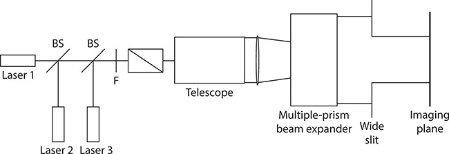
FIGURE 10.19 Three-color industrial PMPML printer used to expose a scale of images at various laser intensities for sensitometric measurements. The telescope expands the beam in two dimensions, whereas the multiple-prism beam expander magnifies in only one dimension parallel to the plane of propagation.
The PMPML printer described in Figure 10.19 uses a single optical channel with a principal laser as the first element defining the optical axis and secondary lasers adding their radiation via beam splitters. All lasers are polarized parallel to the plane of incidence. A variable broadband neutral density filter is inserted as a coarse intensity control prior to the polarizer. The polarizer is a Glan–Thompson prism pair, with an extinction coefficient of 1 × 10⁻⁶ or better, mounted on a high-precision annular rotational stage capable of a 0.001 arc sec angular resolution. As described in Chapter 5, rotation of this polarizer causes the transmission of the lasers to decrease from nearly full transmission to total extinction (Duarte 2001). For the lasers polarized parallel to the plane of propagation, optimum transmission is accomplished with the Glan– Thompson polarizer deployed as depicted in Figure 10.19. Rotation of the polarizer by π/2 radians causes complete extinction of the combined laser beam, and thus no exposure. The use of Glan–Thompson polarizers to vary and fine-tune the intensity of lasers used in laser cooling experiments was reported by Olivares et al. (2009).
Following the polarizer, the beams enter a telescope–lens system and a multiple-prism beam expander as described in Figure 10.1. The elongated near-Gaussian beams are then propagated through a wide aperture so as to produce a diffractive profile as depicted in Figure 10.20. Note that the diffractive profile is wider than the width of the exposures needed so that the intensity variation caused by the ears of the profile does not affect the wanted area. The slight variations toward the center of the distribution have a negligible effect.
Using the method just described, a line exposure is instantaneously printed, thus eliminating the need to displace the laser beams and the associated electromechanical means necessary to accomplish this task. Since the line exposure is horizontal, the imaging material is displaced in a plane orthogonal to the plane of incidence of the instrument. In PMPML printers, the temporal exposures are provided by using the lasers in a pulsed mode. Thus, depending on the lasers, it is possible to vary the exposure time from less than 1 to 1000 ns, thus greatly increasing the range of exposures available for sensitometry and imaging applications (Duarte et al. 2005). It should also be mentioned that careful selection of the beam profiles of the lasers and their respective distances to the main optical axis enables spatial overlapping of the laser beams to within 1 μm at the focal plane with a minimal use of extra beam shaping optics. As indicated by Duarte (2001), lasers suitable for illumination include mode-locked diode-pumped frequency-doubled Nd:YAG lasers and pulsed semiconductor lasers.
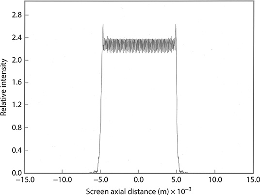
FIGURE 10.20 Diffraction profile of the illumination line at λ = 532 nm.
Problems
10.1 For the telescope, lens, multiple-prism, architecture depicted in Figure 10.1, derive its propagation ray transfer matrix given in Equation 10.9.
10.2 Show that in the absence of a convex lens, Equation 10.9 reduces to Equation 10.16.
10.3 Show that in the absence of a convex lens, Equation 10.15 reduces to Equation 10.17.
10.4 Design a double-prism beam expander yielding zero dispersion at the wavelength of design and M = 5 for an optical system as depicted in Figure 10.1. Using a Galilean telescope with Mt 20, and a convex lens with f = 30 cm, calculate the width and the height of the resulting extremely elongated near-Gaussian beam at the focal plane.
Assume a TEM00 He–Ne laser at λ = 632.82 nm and w0 = 250 μm. For the material of the multiple-prism beam expander, use fused silica.
10.5 For a beam splitter made of fused silica and a thickness of 0.4 mm, determine the lateral displacement, from its original path, of a TEM00 He–Ne laser beam at λ = 632.82 nm, immediately following the beam splitter if the angle of incidence is at the Brewster angle.