
12
Spectrometry
12.1 Introduction
Spectrometry and spectrophotometry are two important subfields that are part of the larger field of optical metrology. Spectrometry mainly utilizes dispersive-based instrumentation that can be based on prismatic configurations, diffraction grating configurations, or a combination of these. The principal exercise here is to obtain a record of intensity versus wavelength of the material of interest, which provides a unique signature for the atomic or molecular structure of the medium under examination. If a tunable, or broadband, light source illuminates a material sample in the transmission mode, as illustrated in Figure 12.1, then a wavelength scan of the spectrometer yields a record of the absorption spectrum. Alternatively, as illustrated in Figure 12.2, a laser-excited atomic or molecular medium can be used to yield a fluorescence spectrum and an emission spectrum.
In Figure 12.3, a fluorescence spectrum from electronic system of the I2 molecule is displayed. This spectrum was generated using a narrow-linewidth tunable laser emitting at λ ≈ 589 nm (Duarte 1981). Here the basics of dispersive spectrometry, or spectrophotometry, are presented, while indicating that most of the recent advancements in this area are related to compactness, miniaturized electronics, digital detector resolution improvements, digital detection wavelength range extensions, digital detector sensitivity improvements, and software augmentations, whereas the optics basics remain the same.
12.2 Spectrometry
Spectrometry, in principle, depends on the interaction of a light beam with a dispersive element, or dispersive elements, and on spatial discrimination following post-dispersive propagation. Hence, the higher the dispersive power, the longer the optical path of the postdispersive propagation, the higher the spatial resolution of the digital detector, the higher the wavelength resolution. As described in earlier chapters, dispersion can be provided by prisms, gratings, or prism–grating combinations. For a detailed treatment on the subject of spectrometry, the reader should refer to the work of Meaburn (1976).
12.2.1 Prism Spectrometers
Prism spectrometry has its origin in the experiments reported by Newton (1704) in his book Opticks. The generalized single-pass multiple-prism dispersion equation (Duarte and Piper 1982, 1983)
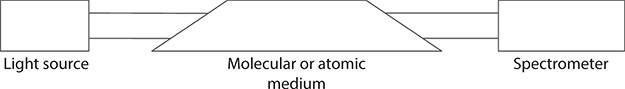
FIGURE 12.1 Simple optical configuration for absorption measurements using a spectrometer.
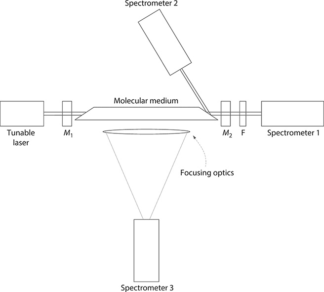
FIGURE 12.2 Simplified optical configuration for fluorescence and emission measurements, in an optically pumped laser system, using spectrophotometers. A narrow-linewidth tunable laser excites longitudinally a molecular medium, such as I2, and the emission is detected by spectrometer 1 via a filter F used to stop residual emission from the pump tunable laser. In addition, the emission can also be detected via the reflection of the Brewster window of the optical cell in spectrometer 2. The fluorescence and emission are detected orthogonally to the optical axis in spectrometer 3 as described by Duarte. (Adapted from Duarte, F.J., Investigation of the Optically-Pumped Iodine Dimer Laser in the Visible, Macquarie University, Sydney, Australia, 1981.)
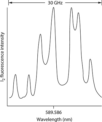
FIGURE 12.3 Fluorescence spectrum of the I2 molecule generated using pulsed narrow-linewidth tunable laser excitation in the vicinity of λ = 589.586 nm. The tuning range is 30 GHz or ~1 cm−1 as described by Duarte. (Data from Duarte, F.J., Investigation of the Optically-Pumped Iodine Dimer Laser in the Visible, Macquarie University, Sydney, Australia, 1981.)
and its explicit version (Duarte 1985, 1990)
can be used to quantify the dispersion of any multiple-prism dispersive arrangement applicable to various instruments of practical interest. This is important since the dispersion determines the linewidth resolution of the instrument via
Prism spectrometers usually deploy equilateral, or isosceles, prisms, in series to augment the dispersion of the instrument. As described in Chapter 4, for an array of r identical isosceles, or equilateral, prisms deployed symmetrically, in an additive configuration, so that ϕ1,1 = ϕ1,2 = ··· = ϕ1,m and ϕ1,m = ϕ2,m, the cumulative dispersion (Equation 12.1) reduces to (Duarte 1990)
and
where all angular parameters are described in Chapter 4. These equations indicate that dispersion can be augmented by a combination of two factors: increasing the number of prisms and using prisms with a high material dispersion. For some materials, ∇λn is given in Table 4.1.
Prism spectrometers assume various configurations. Two of these are considered here. The first configuration, depicted in Figure 12.4, uses two prisms in series with a considerable distance between the two prisms to increase the overall angular spread of the emerging beam. Long postdispersive optical paths, of up to 3 m, in conjunction with narrow apertures, provide wavelength resolutions in the nanometer range. The second architecture, described by Meaburn (1976), includes a sequence of several prisms in series as depicted in Figure 12.5. In this configuration, dispersion is simply augmented by a larger factor r in Equation 12.4. The same observations about the postdispersive optical path, and spatial discrimination, are relevant.
12.2.2 Diffraction Grating Spectrometers
As described in Chapter 2, the diffraction grating equation is given by
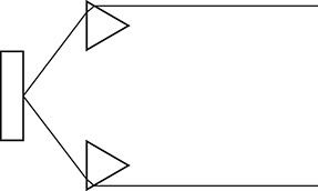
FIGURE 12.4 Long-optical path double-prism spectrometer.
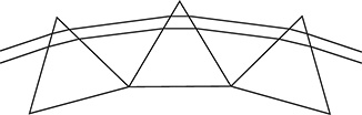
FIGURE 12.5 Dispersive assembly of multiple-prism spectrometer. The angle of incidence ϕ1,m and the angle of emergence ϕ2,m are identical for all prisms. In addition to the cumulative dispersion, resolution is determined by the path length toward the exit slit and the dimensions of the slit.
and, the angular dispersion is obtained by differentiating this equation so that
or alternatively
For a grating deployed in Littrow configuration, Θ = Φ and the grating equation becomes
so that the dispersion can be expressed as
As with prismatic spectrometers, the three factors that increase wavelength resolution in a diffraction grating spectrometer are the dispersion, the optical path length, and the dimensions of the aperture at the detection plane. From Equation 12.7, it is clear that one avenue to increase dispersion is to use gratings deployed at a higher order or to employ gratings with a high groove density. Since deployment of gratings at high orders might lead to a decrease of diffraction efficiency, the alternative of using high-density gratings with 3000 lines/mm, or more, is a practical alternative to increase dispersion. Selection of a particular grating should consider the spectral region of desired operation since high-density gratings might cease to diffract toward the red end of the spectrum. The electromagnetic theory of diffraction gratings is considered in detail by Maystre (1980). A fundamental form of grating spectrometer is shown in Figure 12.6 in order to illustrate the basic concept of spec-trometry. The use of high-dispersion gratings in conjunction with high-resolution digital detectors, as outlined in Figure 12.6b, can lead to the configuration of miniature dispersive spectrometers or wavelength meters. Among the most widely used diffraction grating spectrometer configurations is the Czerny–Turner spectrometer, as shown in Figure 12.7, where two mirrors are used to increase the optical path length, and thus the resolution. A modified Czerny–Turner spectrometer (Meaburn 1976) includes two gratings to increase the dispersion (Figure 12.8). A simple modification to increase resolution is to increase the optical path directly or by adding further stages of reflection. Various spectrometer design alternatives are discussed by Born and Wolf (1999) and Meaburn (1976). It should be noted that the use of curved gratings and curved mirrors to compensate for losses is prevalent in many designs. Notable among the curved grating approaches are the Rowland and the Paschen configurations (Born and Wolf 1999).
Modern Czerny–Turner spectrometer designs, with a ~4 m folded optical path, provide resolutions in the 0.01 nm region, in the visible spectrum, when using slits a few micrometers wide. These spectrometers are very useful in providing the first approach to determine the value of a laser wavelength.

FIGURE 12.6 (a) Basic grating spectrometer. The resolution is mainly determined by the dispersion of the grating, deployed in a non-Littrow configuration, and by the optical path length toward the exit slit (S2). (b) A variation on the basic grating spectrometer consists in deploying a high-dispersion diffraction grating in conjunction with a high spatial resolution digital detector (CCD or CMOS) to register the diffracted light.
12.2.2.1 Example
Using a 3000 lines/mm diffraction grating deployed at Θ = 60.0000°, m = 1, at λ = 590.00 nm, from Equation 12.6
it can be established that the angle of diffraction is Φ = 64.685530°. Next, if the angle of incidence is maintained at Θ = 60.000000° and the wavelength is varied to λ = 590.10 nm, then the angle of diffraction becomes Φ = 64.725759q, so that δΦ = 0.042293 for δλ = 0.10 nm (see Problem 12.3).
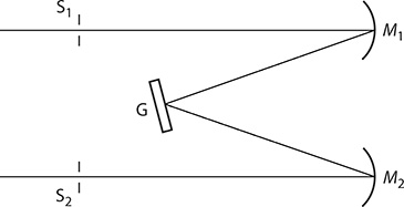
FIGURE 12.7 Czerny–Turner spectrometer. Mirrors M1 and M2 provide the necessary curvature to focus the diffracted beam at the exit slit.
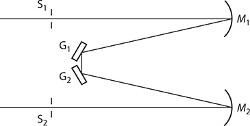
FIGURE 12.8 Double-grating Czerny–Turner spectrometer. Mirrors M1 and M2 provide the necessary curvature to focus the diffracted beam at the exit slit.
12.3 Dispersive Wavelength Meters
Dispersive wavelength meters are in essence dispersive spectrometers with the conventional slit-detector arrangement replaced by a linear photodiode array, charge-coupled device (CCD), or complementary metal–oxide–semiconductor (CMOS) detector. Their main function is to determine the wavelength from the emission of tunable lasers. The resolution is determined by the available dispersion, the propagation distance between the dispersive element and the detector array, and the dimensions of the individual pixels at the digital array. Depending on the type of detector, individual pixels vary in size from a few micrometers to ~25 μm in width. The typical widths of these digital arrays vary from ~25 to ~50 mm. This type of wavelength meter is used in conjunction with well-known, and preferably stabilized, laser sources for calibration. Morris and McIlrath (1979) used a 40 cm spectrometer, incorporating an echelle grating deployed at a high order, in conjunction with a photodiode array integrated by 1024 elements (each ~25 mm wide) to determine wavelengths within 0.01 nm in the visible region.
A wavelength meter based on a high-dispersion prism grating configuration is illustrated in Figure 12.9. As discussed in Chapter 4, the return-pass dispersion of a multiple-prism assembly and a diffraction grating is given by (Duarte and Piper 1982, 1984).
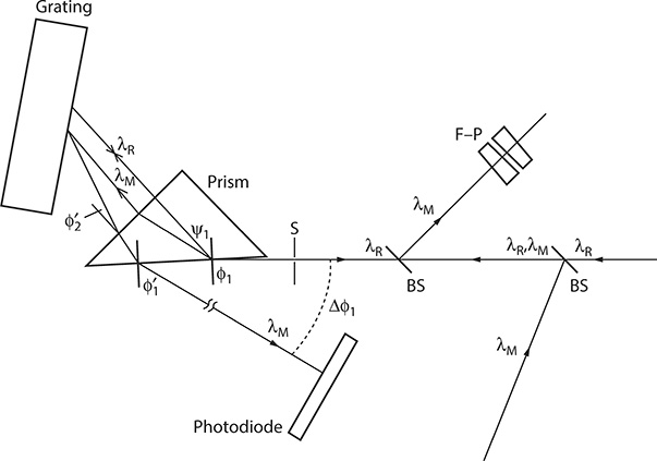
FIGURE 12.9 Architecture of the prism grating wavelength meter. A reference wavelength (λR) beam and the measurement wavelength (λM) beam are combined at the entrance beam splitter (BS). The reference beam is used to provide the initial reference wavelength (λR) and for alignment purposes (λM > λR). A second BS sends light from (λM) beam to a Fabry–Pérot (F–P). The (λM) and (λR) beams are separated at the prism. The (λM) beam undergoes deflection at the prism grating assembly, whereas the (λR) beam returns back on its original path. The measurement beam (λM) undergoes augmented angular deflection at the prism grating system and its position is registered by a photodiode array or CCD. Resolution is a function of the overall prism grating dispersion, the distance between the prism and the photodiode array detector, and the spatial resolution (pixel dimensions) of the digital detector. (Reproduced from Duarte, F.J., J. Phys. E: Sci. Instrum., 16, 599–601, 1983. With permission from the Institute of Physics.)
where:
so that
For a single prism, r = 1, and Equation 12.13 becomes
which, for orthogonal beam exit, that is, ϕ2,1 = ψ2,1 ≈ 0, reduces to
Since for that condition
then we have
where:
∇λΘG is the grating dispersion
∇λϕ2 1, is the single-pass prism dispersion
Equation 12.17 neatly illustrates that the original diffraction grating dispersion ∇λΘG is now multiplied by the beam expansion k11, experienced at the prism and the overall dispersion also adds the contribution by the prism.
Using a 600 lines/mm echelle grating deployed in the third order, and a BK-7 optical glass prism (n = 1.512 at λ = 568.8 nm) with an apex angle of 41.5°, the sensitivity of the system becomes 0.3 nm–1 (Duarte 1983). For a 1000 mm distance, from the prism to the detector, this dispersive combination can measure wavelengths with a 0.01 nm resolution. Absolute wavelength calibration was provided by the spectrum of molecular iodine and the I2 spectral atlas of Gerstenkorn and Luc (1978). Once calibrated, this simple prism grating wavelength meter configuration offers static operation and can be used to characterize either pulsed or continuous-wave laser radiation. Resolution is a function of geometry and the intrinsic resolution of the digital detector employed.
Problems
12.1 Use Equation 12.5 to calculate the overall dispersion of an equilateral 60° prism. The prism is fused silica with n = 1.4583 at λ = 590 nm and assume incidence at the Brewster angle.
12.2 Assume you have three identical fused silica prisms as described in Problem 12.1.
Assume further that these prisms are deployed in series in an additive configuration (see Figure 12.5) for incidence at the Brewster angle. Calculate the overall dispersion of this triple-prism configuration
12.3 For a diffraction grating with 3000 lines/mm, as described in Section 12.2.2.1, calculate the minimum pixel resolution necessary for a linear CCD or CMOS detector to discriminate a wavelength change of δλ = 0.10 nm at Θ = 60.000000° and λ = 590.00 nm. Assume that the digital detector is positioned parallel to the surface of the diffraction grating (see Figure 12.6) at a distance of 20 mm, and that the divergence of the incident beam, with 2w = 10 μm, is negligible.
12.4 For a 600 lines/mm echelle grating deployed in Littrow configuration, at λ1 = 441.563 nm, calculate the angular deviation experienced by a collinear, secondary laser beam, at λ2 = 568.8 nm. Assume m = 3.
12.5 Using the prism grating configuration, depicted in Figure 12.9, estimate the new angular deviation Δϕ1 between two collinear laser beams at λ1 = 441.563 nm and λ2 = 568.8 nm. Assume that the prism has a 41.5° apex angle and that n = 1.512 at λ2 = 568.8. Also assume that the 600 lines/mm echelle grating is deployed in Littrow configuration, for the shorter wavelength, at m = 3.