
11
Interferometry
11.1 Introduction
In this chapter, some widely applied interferometric configurations in the measurement of wavelength and linewidth are described. Attention is focussed on two-beam, and multiple-beam, interferometers. See Steel (1967) for a detailed treatment on the subject of interferometry. The presentation given here follows that of the first edition of Tunable Laser Optics (Duarte 2003) while adopting modifications and improvements introduced mainly in the work of Duarte (2014).
11.2 Two-Beam Interferometers
Two-beam interferometers are optical devices that divide and then recombine a light beam. It is on recombination of the beams that interference occurs. The most well-known two-beam interferometers are the Sagnac interferometer, the Mach–Zehnder interferometer, and the Michelson interferometer. For a highly coherent light beam, such as the beam from a narrow-linewidth laser, the coherence length
can be rather large, thus allowing a relatively large optical path length in the two-beam interferometer of choice. Alternatively, this relation provides an avenue to accurately determine the linewidth of a laser by increasing the optical path length until interference ceases to be observed.
11.2.1 The Sagnac Interferometer
The Sagnac, or cyclic, interferometer is illustrated in Figure 11.1. In this interferometer, the incident light beam is divided into two sub-beams by a beam splitter (BS). The reflected beam, on the incidence BS, is then sent into a path defined by the reflections on M1, M2, and M3 mirrors. The transmitted beam, on the incidence BS, is sent into a path defined by the reflections on M3, M2, and M1 mirrors. Both counter-propagating beams are recombined at the BS. The interference mechanics of the counter-propagating round trips can be described using Dirac’s notation via the probability amplitude:
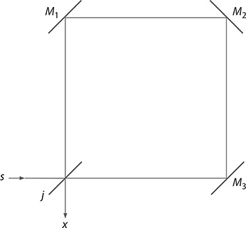
FIGURE 11.1 Sagnac interferometer. All three mirrors M1, M2, and M3 are assumed to be identical.
where:
j refers to the reflection mode of the BS
j′ refers to the transmission mode of the BS
Assuming that
and
Then, Equation 11.2 reduces to
If j′ = 1 represents the BS in the transmission mode and j = 2 in the reflection mode, then Equation 11.5 can be written as (Duarte 2003)
which, for N = 2, can be expressed as
An alternative triangular Sagnac interferometer, with only two mirrors (M1 and M2), is shown in Figure 11.2.

FIGURE 11.2 Triangular Sagnac interferometer.
11.2.2 The Mach-Xehnder Interferometer
The Mach–Zehnder interferometer is illustrated in Figure 11.3. In this interferometer, the incident light beam is divided into two sub-beams by a BS. The reflected beam, on the incidence BS, is then sent into a path defined by the reflection on M1 toward the exit BS. The transmitted beam, on the incidence BS, is sent into a path defined by the reflection on M2 toward the exit BS. Both counter-propagating beams are recombined at the exit BS. The interference mechanics of the counter-propagating beams can be described using Dirac’s notation via the probability amplitude
which can be abstracted to

FIGURE 11.3 Mach–Zehnder interferometer.
If j′ = k′ = 1 represents the BS in the transmission mode and j = k = 2 in the reflection mode, then Equation 11.9 can be written as (Duarte 2003)
The same result can be obtained from
which leads to
However, since 〈1 | 1〉 and 〈2 | 2〉 illuminate x′ rather than x, the probability amplitude, for this geometry, reduces to that given in Equation 11.10.
A prismatic Mach–Zehnder interferometer is illustrated in Figure 11.4. In this prismatic version of the Mach–Zehnder, there is asymmetry in regard to the intra-interferometric beam dimensions. The P1 – M2 – P2 beam is expanded relatively to the P1 – M1 – P2 beam. Also, in this particular example (based on a prism with a magnification of k1,1 ≈ 5), there is also a power asymmetry since the unexpanded beam propagating in the P1 – M1 – P2 arm has about 30% of the incident power, whereas the expanded beam P1 – M2 – P2 carries the remaining 70% of the incident power, for light polarized parallel to the plane of incidence. In this regard, it should be possible to design a prismatic Mach–Zehnder where the power density (W m−2) in each arm is balanced. Applications for this type of interferometer include imaging and microscopy. Additional Mach–Zehnder interferometric configurations include transmission gratings as BS (Steel 1967).
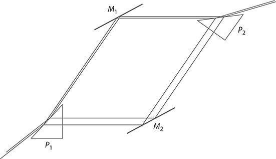
FIGURE 11.4 Prismatic Mach–Zehnder interferometer. (Reproduced from Duarte, F.J., Quantum Optics for Engineers, CRC Press, New York, 2014. With permission.)
11.2.3 The Michelson Interferometer
The Michelson interferometer (Michelson 1927) is illustrated in Figure 11.5. In this interferometer, the incident light beam is divided into two sub-beams by a BS that serves as both input and output elements. The reflected beam, on the incidence BS, is then sent into a path defined by the reflection on M1 and back toward the exit BS. The transmitted beam, on the incidence BS, is sent into a path defined by the reflection on M2 and back toward the exit BS. Both beams are recombined interferometrically at the BS. For the Michelson interferometer, the interference can be characterized using a probability amplitude of the form:
which can be abstracted to
If j′ = 1 represents the function of the BS in the transmission mode and j = 2 in the reflection mode:
It is clear that substitution of the appropriate wave functions for the various terms in Equations 11.5, 11.9, and 11.14, and multiplication of these equations with their respective complex conjugates yield probability equations of an interferometric character. A variant of the Michelson interferometer uses retroreflectors (Steel 1967).
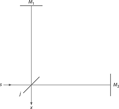
FIGURE 11.5 Michelson interferometer.
11.3 Multiple-Beam Interferometers
An N-slit interferometer, which can be considered as a multiple-beam interferometer, was introduced in Chapter 2 and is depicted in Figure 11.6. In this configuration, an expanded beam of light illuminates simultaneously N slits. Following propagation, the N sub-beams interfere at a plane perpendicular to the plane of propagation. The probability amplitude is given by the Dirac principle
and the probability is
which can also be expressed as (Duarte 1991, 1993)
The explicit expansion of the above equation for higher values of N is illustrated in Chapter 2. Two-dimensional and three-dimensional versions of Equation 11.18 are also given in Chapter 2.

FIGURE 11.6 N-slit interferometer. CMOS, complementary metal–oxide–semiconductor; TEM00, single transverse mode.
11.3.1 The Hanbury Brown–Twiss Interferometer
The Hanbury Brown–Twiss effect originates in interferometric measurements performed by an intensity interferometer used for astronomical observations (Hanbury Brown and Twiss, 1956). A diagram of the stellar intensity interferometer used to determine the diameter of stars is depicted in Figure 11.7. Feynman in one of his exercises to The Feynman Lectures on Physics (Feynman et al. 1965) explains that the electrical currents from the two detectors are mixed in a coincidence circuit where the currents become indistinguishable. Feynman then asks to show that the coincidence counting rate, in the Hanbury Brown–Twiss configuration, is proportional to an expression of the form:
where:
R1 and R2 are the distances from detector 1 and detector 2 to the source
Using the N-slit interferometric equation (Duarte 1991, 1993), that is, Equation 11.18, with N = 2, one immediately arrives at
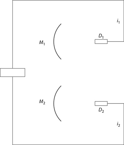
FIGURE 11.7 The Hanbury Brown and Twiss interferometer. The light, from an astronomical source, is collected at mirrors M1 and M2 and focused onto detectors D1 and D2. The current generated at these detectors, i1 and i2, interfere at the electronics to produce an interference signal characterized by an equation of the form of Equation 11.18 with N = 2.
and setting Ψ(r1) = Ψ(r2) = 1
Now, using (as suggested by Feynman) Ω1 = kR1 and Ω2 = kR2
which is the result given by Feynman in his problem book (Feynman 1965). From the measured signal distribution, and these equations, the angular spread of the emission can be determined, and knowing the distance from the source to the detector, it becomes possible to estimate the diameter of the aperture at the emission, in other words, the diameter of the star under observation.
Finally, since all the physics of the Hanbury Brown–Twiss interferometer follows from the generalized interferometric equation:
it can be easily seen that the experimental arrangement of the astronomical telescope should not be limited to just two parabolic mirrors and two detectors (N = 2), but can be extended to an array of N parabolic mirrors with their corresponding detectors.
11.3.2 The Fabry–Pérot interferometer
The second multiple-beam interferometer is the Fabry–Pérot interferometer depicted in Figure 11.8. This interferometer has already been introduced in Chapter 7 as an intracavity etalon. Generally, intracavity etalons are a solid slab of optical glass, or fused silica, with highly parallel surfaces coated to increase reflectivity (Figure 11.8b). These are also known as Fabry–Pérot etalons. Fabry–Pérot interferometers, however, are constituted by two separate slabs of optical flats with their inner surfaces coated as shown in Figure 11.8a. The space between the two coated surfaces is filled with air or other inert gas. The optical flats in a Fabry–Pérot interferometer are mounted on rigid metal bars, with a low thermal expansion coefficient, such as Invar. The plates can be moved, with micrometer precision or better, to vary the free spectral range (FSR). These interferometers are widely used to characterize and quantify the laser linewidth.
The mechanics of multiple-beam interferometry can be described in some detail, considering the multiple reflection, and refraction, of a beam incident on two parallel surfaces separated by a region of refractive index n as illustrated in Figure 11.9. In this configuration, at each point of reflection and refraction, a fraction of the beam, or a sub-beam, is transmitted toward the boundary region. Following propagation, these sub-beams interfere. In this regard, the physics is similar to that of the N-slit interferometer with the exception that each parallel beam has less intensity due to the increasing number of reflections. Here, for transmission, interference can be described using a series of probability amplitudes representing the events depicted in Figure 11.9

FIGURE 11.8 Fabry–Pérot interferometer (a) and Fabry–Pérot etalon (b). Dark lines represent coated surfaces. Focusing optics is often used with these interferometers when used in linewidth measurements.

FIGURE 11.9 Multiple-beam interferometer: (a) Multiple internal reflection diagram; (b) detailed view depicting the angles of incidence and refraction.
where:
j is at the reflection surface of incidence
k is immediately next to the surface of reflection
l is at the second surface of reflection
m is immediately next to the second surface of reflection as illustrated in Figure 11.9
The problem can be simplified considerably if the incident beam is considered as a narrow beam incident at a single point j. Propagation of the single beam then proceeds to l and is represented by the incidence amplitude Ai, which is a complex number, attenuated by the transmission factor t, so that the first three probability amplitudes can be represented by an expression of the form:
and Equation 11.23 reduces to
which, using the notation of Born and Wolf (1999), can be expressed as
defining
and
and taking the limit as p → ∞, Equation 11.25 reduces to (Born and Wolf 1999)
and multiplication with its complex conjugate yields an expression for the intensity
which is known as the Airy formula or Airy function. Plotting the ratio of the two intensities, as a function of
shows that the contrast of the fringes increases as the reflectivity increases (Born and Wolf 1999). From the geometry of Figure 11.9b, the path difference between the first reflected beam and the first beam that undergoes internal reflection, followed by refraction, is (see Problem 11.4)
which reduces to
Hence, using ΔL = mλ, the path difference can be expressed as
where:
n is the refractive index of the medium
de is the distance between the reflection surfaces
It also follows that the phase difference, using Equations 11.31 and 11.33, can be found to be
The device just described is an uncoated interferometer. If the two surfaces of the plate are coated with metal films of equal reflectivity, the phase term is modified so that (Born and Wolf 1999)
where:
ϕ represents a phase change
Under these circumstances, the multiple-beam interferometer is classified as a Fabry–Pérot etalon. An interferogram produced by the interaction of narrow-linewidth laser emission and a Fabry–Pérot etalon followed by a convex lens, of focal length f, is shown in Figure 11.10.
Using δ = 2πm in Equation 11.36, we get
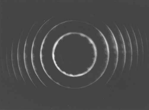
FIGURE 11.10 Fabry–Pérot interferogram depicting single-longitudinal-mode oscillation, at Δν ≈ 700 MHz, from a tunable multiple-prism grating solid-state oscillator. (Reprinted from Opt. Commun., 117, Duarte, F.J., Solid-sate dispersive dye laser oscillator: Very compact cavity, 480–484, Copyright 1995, with permission from Elsevier.)
Here, the brightest central ring corresponds to the maximum value of m0, which is
which can be expressed as
where:
ε is the fractional fringe order
Using these equations, the diameter of the rings is given by (Born and Wolf 1999)
where:
p = 1, 2, 3... enumerates the successive rings from the center
11.3.3 Design of Fabry–Pérot Etalons
The FSR of a Fabry–Pérot interferometer, or a Fabry–Pérot etalon, corresponds to the difference in wavelength of two adjacent orders. From Equation 11.34, for a small angle of incidence,
and for an infinitesimal wavelength difference, corresponding to two adjacent orders, Δm becomes
Since Δm = 1, the wavelength difference corresponds to
which has the same form of Δλ ≈ λ2 / Δx derived in Chapter 3 from interferometric principles while discussing Heisenberg’s uncertainty principle.
Renaming the wavelength difference as the FSR, we can write
which in the frequency domain becomes
Here, the approximations δλ ≈ (λ1 − λ2) and λ2 ≈ λ1λ2 are justified since λ >> Δλ.
The FSR corresponds to the separation of the rings in Figure 11.10 and a measure of the width of the rings determines the linewidth of the emission being observed. The minimum resolvable linewidth is given by
where:
ℱ is the effective finesse.
Thus, a Fabry–Pérot etalon with an FSRe = 7.49 GHz and F = 50 provides discrimination down to ΔνFRS ≈ 150 MHz. The finesse is a function of the flatness of the surfaces (often in the λ/100−λ/50 range), the dimensions of the aperture, and the reflectivity of the surfaces. The effective finesse is given by (Meaburn 1976)
where:
ℱR, ℱF, and ℱA are the reflective, flatness, and aperture finesses, respectively
The reflective finesse is given by (Born and Wolf 1999)
11.3.3.1 Example
A Fabry–Pérot etalon, with de = 10.27 mm and capable of resolving laser linewidths down to Δνe ≈ 100 MHz, needs to be coated with only the necessary reflectivity. The flatness of the surfaces is λ/100, the material is fused silica (n = 1.4583 at λ = 590 nm), and the dominating finesse parameter is FR. With this information, it is found that
which, from Equation 11.48, requires R ≈ 0.97.
11.4 Coherent and Semicoherent Interferograms
The topic of coherence and semicoherence of N-slit interferograms is discussed in more detail by Duarte (2014). Here, a summary of the main concepts is given.
The generalized interferometric equation in one dimension
was derived for single-photon propagation (Duarte 1991, 1993, 2004), which means that, strictly speaking, it applies only to monochromatic sources. To emphasize this point, this equation should really be written as (Duarte 2014)
In practice, however, it has been found that this equation can be applied to either reproduce or predict N-slit interferograms generated using narrow-linewidth lasers that emit ensembles of indistinguishable photons (Duarte 1993). These interfero-grams are characterized by sharp well-defined features with a high degree of visibility as defined by (Michelson 1927)
Also, from experiments, we know that broadband light sources produce N-slit inter-ferograms with broad features that are characterized by lack of sharpness (Duarte 2007, 2008, 2010). As explained in Duarte (2014), interferograms produced with broadband light are generated by a multitude of wavelengths, and the digital detector, or photographic plate, used to record the interference yields an integrated version of a multitude of interferograms, all of which have different interferometric features. Therefore, interferograms generated using non-narrow-linewidth emission, or broadband radiation, have broad features and low visibility as defined by Equation 11.50 (see Figure 11.11). Thus, the correct interferometric equation for semicoherent radiation, and broadband radiation, is modified to include a sum over the wavelength range involved so that (Duarte 2014)
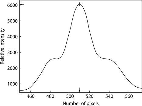
FIGURE 11.11 Measured double-slit (N = 2) interferogram generated with a broadband light source. The slits are 50 μm wide separated by 50 μm and D〈x | j〉 10 cm. Comparison with other two-slit interferograms generated with coherent sources (see Figures 11.12 and 11.13) reveals lack of spatial definition and low visibility as defined by Equation 11.50.
From a computational perspective, the broadly featured interferogram can be approximated via the generation of a large number of single-wavelength interferograms at fine intervals of wavelength. Each of these interferograms will have slightly different intensity-spatial features and the overall interferometric profile will be an integrated, or cumulative, interferogram.
11.4.1 Example
In Figure 11.12, the double-slit interferogram produced with narrow-linewidth emission from the 3s2 - 2p10 transition of a He–Ne laser, at λ ≈ 543.3 nm, is displayed. The visibility of this interferogram is calculated, using Equation 11.50, to be V ≈ 0.95. In Figure 11.13, the double-slit interferogram produced, under identical geometrical conditions, but with the emission from an electrically excited coherent organic semiconductor interferometric emitter (Duarte et al. 2005), at λ ≈ 540 nm,
is displayed. Here, the visibility is lower (V ≈ 0.90). A comparison between the two interferograms reveals that the second interferogram has slightly broader spatial features relative to the interferogram produced with illumination from the 3s2 - 2p10 transition of the He–Ne laser. The differences in spatial distributions between these two interferograms have been used to estimate the linewidth of the emission from the interferometric emitter (Duarte 2008).
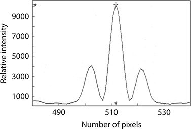
FIGURE 11.12 Double-slit interferogram from the narrow-linewidth emission from the 3s2 - 2p10 transition of a He–Ne laser, at λ ≈ 543.3 nm. The visibility of this interferogram is V ≈ 0.95. Here, N = 2, the slits are 50 μm wide separated by 50 μm, and D〈x | j〉 = 5cm. (Reproduced from Duarte, F.J., et al., Opt. Lett., 30, 3072–3074, 2005. With permission from the Optical Society.)

FIGURE 11.13 Double-slit interferogram from an electrically excited organic semiconductor interferometric emitter at λ ≈ 540 nm. The visibility of this interferogram is less than V ≈ 0.90. Here, N = 2, the slits are 50 μm wide separated by 50 μm, and D〈x | j〉 = 5cm. (Reproduced from Duarte, F.J., et al., Opt. Lett., 30, 3072–3074, 2005. With permission from the Optical Society.)
11.5 Interferometric Wavelength Meters
Interferometric signals and profiles are a function of the wavelength of the radiation that produces them. Thus, interferometers are well suited to be applied as wavelength meters, especially when a digital detector array is used to record the resulting interferogram. As such, a variety of interferometric configurations have been used in the measurement of tunable laser wavelengths. For a review in this subject, the reader should refer to the work of Demtröder (2008).
The wavelength sensitivity of multiple-beam interferometry has its origin in the phase information of the equations describing the behavior of the interferometric signal. In the case of the N-slit interferometer, the interferometric profile is characterized by Equation 11.18, which includes a phase difference term that, as explained in Chapter 2, can be expressed as
where:
and
where:
λv is the vacuum wavelength
n1 and n2 are the corresponding indexes of refraction
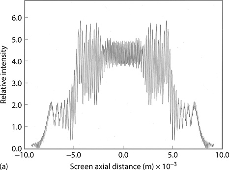
FIGURE 11.14 Interferograms at λ1 = 580 nm (a), λ2 = 585 nm (b), λ3 = 590 nm (c), and nm (d). These calculations are for slits 100 μm wide, separated by 100 μm, and N = 50. The j-to-x distance is D〈x | j〉 = 100 cm.
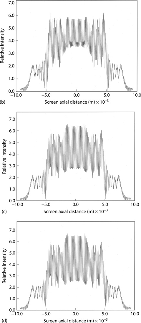
Here, λ1 = λv /n1 and λ2 = λv /n2 (Wallenstein and Hänsch 1974; Born and Wolf 1999). See Chapter 2 for further details. Hence, it is easy to see that different wavelengths will produce different interferograms. To illustrate this point in Figure 11.14, four calculated interferograms, using Equation 11.18, for the N-slit interferometer, with N = 50, are shown. For a given set of geometrical parameters, measured interferograms can be matched, in an iterative process, with theoretical interference patterns to determine the wavelength of the radiation. Again, resolution depends on the optical path length between the slit array and the digital detector, and on the size of the pixels and the linearity of the detector.
11.5.1 Fabry–Pérot Wavelength Meters
For a multiple-beam interferometer, the transmission intensity is given by Equation 11.30, where, in reference to Figure 11.9, the phase term δ can be expressed by Equation 11.36, which depends on the reciprocal of the wavelength. Thus, recording of the transmission interferometric signal by a photodiode array, or charge-coupled device (CCD), yields information on the wavelength of the radiation being measured.
Wavelength meters based on Fabry–Pérot interferometers generally involve configurations with multiple etalons in parallel (Byer et al. 1977; Fischer et al. 1981; Konishi et al. 1981). In the multiple-etalon configuration depicted in Figure 11.15, each etalon has a different FSR that is compatible with the FSR and the finesse of the next etalon. For instance, Fischer et al. (1981) used three etalons with FSRs of 1000, 67, and 3.3 GHz. Briefly, the methodology of this measurement consists in the application of Equations 11.38 and 11.39 to determine λ with reduced uncertainty at each etalon. Using this approach, Fischer et al. (1981) reported the measurements of laser frequencies with an accuracy of 60 MHz.
A simple interferometric configuration that is widely used in the measurement of laser wavelengths is that of the Fizeau, or optical wedge, two-beam interferometer first introduced by Snyder (1977). In this configuration, the incident laser beam propagates on an axis that is at an angle to the optical axis of the digital detector (see Figure 11.16). Also, the incident beam illuminates a wide area of the interferometer using some beam expansion method in conjunction with a spatial filter. The interference of the two beams is recorded by a digital detector with a 25 μm resolution or better. The method employs two predetermined parameters: the angle of the wedge and the wedge separation at a reference position as shown in Figure 11.16b.
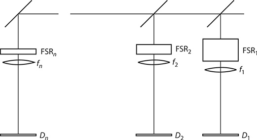
FIGURE 11.15 Multiple-etalon wavelength meter.

FIGURE 11.16 (a) Fizeau wavelength meter. (b) Geometrical details of a Fizeau interferometer.
The spacing of the Fizeau fringes Δz provides an approximate value for the wavelength according to
Assuming a very small wedge angle,
and
so that (Demtröder 2008)
thus allowing the determination of the order of interference at a minimum. The method then compares, using a computer program, the periodicity of the interference pattern with that predetermined from two-beam interference intensity functions. As indicated in Equation 11.18, these interferometric functions depend on the cosine of a phase term that, in this case, depends on Δz, which in turn is a function of the wavelength and the geometry of the wedge. Thus, accurate calibration of the spacing of the wedge allows a determination of the wavelength compatible with the accuracy to which the angle α is known. This static two-beam interferometric approach offers a wide wavelength range and an accuracy better than two parts in 106 (Gardner 1985) in very compact configurations.
Problems
11.1 A laser beam fails to provide interference fringes when the distance from the BS to the mirrors, in a Michelson interferometer, is 1 m. Estimate the linewidth of the laser.
11.2 Use the usual complex-wave representation for probability amplitudes and Equation 11.10 to arrive at an equation for the probability of transmission in a Mach–Zehnder interferometer.
11.3 List the simplifying assumptions that lead from Equation 11.23 through 11.26.
11.4 Use the geometry of Figure 11.9 to derive Equation 11.32.
11.5 Use Equation 11.50 to estimate the visibility of the two-slit interferogram displayed in Figure 11.11.