Chapter 5 Polarization

Search in book...
Toggle Font Controls
Create new playlist

Name your new playlist

Playlist description (optional)
Sign In

Email address

Password

Forgot Password?

or

Continue with Facebook

Continue with Google
Sign Up

Full Name

Email address

Confirm Email Address

Password

or

Continue with Facebook

Continue with Google

This chapter is a revised version of Chapter 5 on classical linear polarization published in Duarte (2003) and includes some new subject matter on polarization as discussed in Duarte (2014).

5.2 Maxwell Equations

Maxwell equations are of fundamental importance since they describe the whole of classical electromagnetic phenomena. From a classical perspective, light can be described as waves of electromagnetic radiation. As such, Maxwell equations are very useful to illustrate a number of the characteristics of light including polarization. It is customary to just state these equations without derivation. Since our goal is simply to apply them, the usual approach will be followed. However, for those interested, it is mentioned that a derivation by Dyson (1990) attributed to Feynman is available in the literature. Maxwell equations in the rationalized metric system are given by (Feynman et al. 1965)

\nabla \cdot B = 0 (5.1)

$\nabla \cdot B = 0 (5.1)$

\nabla \cdot E = \frac{ρ}{ε_{0}} (5.2)

$\nabla \cdot E = \frac{ρ}{ε_{0}} (5.2)$

c^{2} \nabla \times B = \frac{\partial E}{\partial t} + \frac{j}{ε_{0}} (5.3)

$c^{2} \nabla \times B = \frac{\partial E}{\partial t} + \frac{j}{ε_{0}} (5.3)$

\nabla \times E = - \frac{\partial B}{\partial t} (5.4)

$\nabla \times E = - \frac{\partial B}{\partial t} (5.4)$

These equations illustrate, with succinct beauty, the unique coexistence of the electric field and the magnetic field in nature. The first two equations give the value of the given flux through a closed surface, whereas the second two equations give the value of a line integral around a loop. In this notation,

\nabla = (\frac{\partial}{\partial x}, \frac{\partial}{\partial y}, \frac{\partial}{\partial z}) (5.5)

$\nabla = (\frac{\partial}{\partial x}, \frac{\partial}{\partial y}, \frac{\partial}{\partial z}) (5.5)$

where:

E is the electric vector

B is the magnetic induction

ρ is the electric charge density

j is the electric current density

ɛ₀ is the permittivity of free space

c is the speed of light (see Chapter 13)

In addition to Maxwell equations, the following identities are useful:

j = σ E (5.6)

$j = σ E (5.6)$

D = ε E (5.7)

$D = ε E (5.7)$

B = μ H (5.8)

$B = μ H (5.8)$

where:

D is the electric displacement

H is the magnetic vector

σ is the specific conductivity

ɛ is the dielectric constant (or permittivity)

μ is the magnetic permeability

In the Gaussian systems of units, Maxwell equations are given in the form of (see, e.g., Born and Wolf 1999)

\nabla \cdot B = 0 (5.9)

$\nabla \cdot B = 0 (5.9)$

\nabla \cdot E = 4 π p (5.10)

$\nabla \cdot E = 4 π p (5.10)$

\nabla \times H = \frac{1}{c} (\frac{\partial D}{\partial t} + 4 π j) (5.11)

$\nabla \times H = \frac{1}{c} (\frac{\partial D}{\partial t} + 4 π j) (5.11)$

\nabla \times E = - \frac{1}{c} \frac{\partial B}{\partial t} (5.12)

$\nabla \times E = - \frac{1}{c} \frac{\partial B}{\partial t} (5.12)$

It should be noted that many authors in the field of optics prefer to use Maxwell equations in the Gaussian system of units. As explained by Born and Wolf (1999), in this system E, D, j, and ρ are measured in electrostatic units, whereas H and B are measured in electromagnetic units.

For the case of no charges or currents, that is, j = 0 and ρ = 0, and a homogeneous medium, Maxwell equations and the given identities can be applied in conjunction with the vector identity

\nabla \times \nabla \times E = \nabla \nabla \cdot E - \nabla^{2} E (5.13)

$\nabla \times \nabla \times E = \nabla \nabla \cdot E - \nabla^{2} E (5.13)$

to obtain wave equations of the form (Born and Wolf 1999):

\nabla^{2} E - \frac{ε μ}{c^{2}} \frac{\partial^{2} E}{\partial t^{2}} = 0 (5.14)

$\nabla^{2} E - \frac{ε μ}{c^{2}} \frac{\partial^{2} E}{\partial t^{2}} = 0 (5.14)$

This leads to an expression for the velocity of propagation:

v = c (ε μ)^{- 1 / 2} (5.15)

$v = c (ε μ)^{- 1 / 2} (5.15)$

Comparison of this expression with the law of positive refraction, derived in Chapter 4, leads to what is known as Maxwell’s formula (Born and Wolf 1999):

n = (ε μ)^{1 / 2} (5.16)

$n = (ε μ)^{1 / 2} (5.16)$

where:

n is the refractive index

It is useful to note that in vacuum

c^{2} = (ε_{0} μ_{0})^{- 1} (5.17)

$c^{2} = (ε_{0} μ_{0})^{- 1} (5.17)$

in the rationalized metric system, where P₀ is the permeability of free space (Lorrain and Corson 1970). The values of fundamental constants are listed in Chapter 13.

5.3 Polarization and Reflection

Following the convention of Born and Wolf (1999), we consider a reflection boundary, depicted in Figure 5.1, and a plane of incidence established by the incidence ray and the normal to the reflection surface. Here, the reflected component ℛ_|| is parallel to the plane of incidence and the reflected component ℛ_⊥ is perpendicular to the plane of incidence.

Images

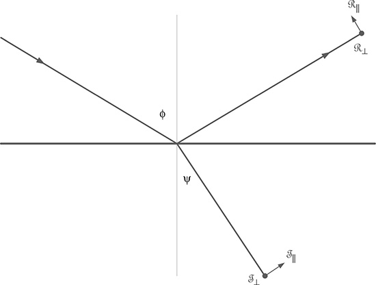
FIGURE 5.1 Reflection boundary defining the plane of incidence. Sometimes, the plane of incidence is also referred to as the plane of propagation.

For the case of μ₁ = μ₂ =1, Born and Wolf (1999) consider the electric, and magnetic, vectors as complex plane waves. In this approach, the incident electric vector is represented by the equations of the form:

E_{x}^{(i)} = - A_{||} \cos (ϕ (e^{- i τ_{i}}) (5.18)

$E_{x}^{(i)} = - A_{||} \cos (ϕ (e^{- i τ_{i}}) (5.18)$

E_{y}^{(i)} = - A_{⊥} (e^{- i τ_{i}}) (5.19)

$E_{y}^{(i)} = - A_{⊥} (e^{- i τ_{i}}) (5.19)$

E_{Z}^{(i)} = - A_{||} \sin (ϕ (e^{- i τ} i) (5.20)

$E_{Z}^{(i)} = - A_{||} \sin (ϕ (e^{- i τ} i) (5.20)$

where:

A_|| and A_⊥ are complex amplitudes

τ_iis the usual plane wave phase factor

Using corresponding equations for E and H for transmission and reflection in conjunction with Maxwell’s relation, with μ = 1, and the law for positive refraction, Born and Wolf (1999) derive the Fresnel formulae:

?_{||} = [\frac{2 \sin ψ \cos (ϕ}{\sin ((ϕ) + ψ) \cos ((ϕ - ψ)}] A_{||} (5.21)

$?_{||} = [\frac{2 \sin ψ \cos (ϕ}{\sin ((ϕ) + ψ) \cos ((ϕ - ψ)}] A_{||} (5.21)$

?_{⊥} = [\frac{2 \sin ψ \cos (ϕ}{\sin ((ϕ + ψ)}] A_{⊥} (5.22)

$?_{⊥} = [\frac{2 \sin ψ \cos (ϕ}{\sin ((ϕ + ψ)}] A_{⊥} (5.22)$

ℛ_{||} = [\frac{\tan ((ϕ) - ψ)}{\tan ((ϕ) + ψ)}] A_{||} (5.23)

$ℛ_{||} = [\frac{\tan ((ϕ) - ψ)}{\tan ((ϕ) + ψ)}] A_{||} (5.23)$

ℛ_{||} = [\frac{\sin ((ϕ) - ψ)}{\sin ((ϕ + ψ)}] A_{⊥} (5.24)

$ℛ_{||} = [\frac{\sin ((ϕ) - ψ)}{\sin ((ϕ + ψ)}] A_{⊥} (5.24)$

Using these equations, the transmissivity and reflectivity for both polarizations can be expressed as

?_{||} = [\frac{(\sin 2_{t} ϕ) \sin 2 ψ)}{\sin^{2} ((ϕ + ψ) \cos^{2} ((ϕ - ψ)}] (5.25)

$?_{||} = [\frac{(\sin 2_{t} ϕ) \sin 2 ψ)}{\sin^{2} ((ϕ + ψ) \cos^{2} ((ϕ - ψ)}] (5.25)$

?_{⊥} = [\frac{(\sin 2_{t} ϕ \sin 2 ψ)}{\sin^{2} ((ϕ) + ψ)}] (5.26)

$?_{⊥} = [\frac{(\sin 2_{t} ϕ \sin 2 ψ)}{\sin^{2} ((ϕ) + ψ)}] (5.26)$

ℛ_{||} = [\frac{\tan^{2} ((ϕ - ψ)}{\tan^{2} ((ϕ) + ψ)}] (5.27)

$ℛ_{||} = [\frac{\tan^{2} ((ϕ - ψ)}{\tan^{2} ((ϕ) + ψ)}] (5.27)$

ℛ_{||} = [\frac{\sin^{2} ((ϕ) - ψ)}{\sin^{2} ((ϕ) + ψ)}] (5.28)

$ℛ_{||} = [\frac{\sin^{2} ((ϕ) - ψ)}{\sin^{2} ((ϕ) + ψ)}] (5.28)$

and

ℛ_{||} + ?_{||} = 1 (5.29)

$ℛ_{||} + ?_{||} = 1 (5.29)$

ℛ_{⊥} + ?_{⊥} = 1 (5.30)

$ℛ_{⊥} + ?_{⊥} = 1 (5.30)$

Using these expressions for transmissivity and reflectivity, the degree of polarization, ?, is defined as (Born and Wolf 1999)

? = \frac{(ℛ_{| |} - ℛ_{⊥})}{(ℛ_{| |} + ℛ_{⊥})} (5.31)

$? = \frac{(ℛ_{| |} - ℛ_{⊥})}{(ℛ_{| |} + ℛ_{⊥})} (5.31)$

The usefulness of these equations is self-evident once ℛ_|| is calculated, as a function of angle of incidence (Figure 5.2), for fused silica at λ ≈ 590 nm (n = 1.4583). Here, we see that ℛ_|| = 0 at 55.5604°. At this angle, (ϕ + ψ) becomes 90° so that tan(ϕ + ψ) approaches infinity, thus causing ℛ_|| = 0. This particular ϕ is known as the Brewster angle (ϕ_B) and has a very important role in laser optics. Since at ϕ = ϕ_B the angle of refraction becomes ψ = (90 − ϕ) degrees and the law of positive refraction takes the form of

\tan ϕ_{B} = n (5.32)

$\tan ϕ_{B} = n (5.32)$

Images

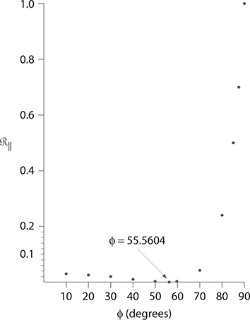
FIGURE 5.2 Reflection intensity as a function of angle of incidence. The angle at which the reflection vanishes is known as the Brewster angle.

For orthogonal, or normal, incidence, the difference between the two polarizations vanishes. Using the law of positive refraction and the appropriate trigonometric identities, in Equations 5.25 through 5.28, it can be shown that (Born and Wolf 1999)

ℛ = [\frac{(n - 1)}{(n + 1)}]^{2} (5.33)

$ℛ = [\frac{(n - 1)}{(n + 1)}]^{2} (5.33)$

? = [\frac{4 n}{(n + 1)}]^{2} (5.34)

$? = [\frac{4 n}{(n + 1)}]^{2} (5.34)$

5.3.1 Plane of Incidence

The discussion in Section 5.3 uses parameters such as ℛ_|| and ℛ_⊥. In this convention, & means parallel to the plane of incidence and ⊥ means perpendicular, orthogonal, or normal to the plane of incidence. The plane of incidence is defined, following Born and Wolf (1999), in Figure 5.1. This plane can also be referred to as the plane of propagation.

On more explicit terms, let us consider a laser beam propagating on a plane parallel to the surface of an optical table. If that beam is made to illuminate the hypotenuse of a right-angle prism, whose triangular base is parallel to the surface of the table, then the plane of incidence is established by the incident laser beam and perpendicular to the hypotenuse of the prism. In other words, in this case, the plane of incidence is parallel to the surface of the optical table. Moreover, if that prism is allowed to expand the transmitted beam, as discussed later in this chapter, then the beam expansion is parallel to the plane of incidence.

The linear polarization of a laser can often be orthogonal to an external plane of incidence. When this is the case, and the maximum transmission of the laser through external optics is desired, either the laser is rotated by π/2 about its axis of propagation, or a collinear π/2 polarization rotator is used as discussed later in this chapter.

5.4 Jones Calculus

Jones calculus is a matrix approach to describe, in a unified form, both linear and circular polarization. It was introduced by Jones (1947) and a good review of the subject was given by Robson (1974). Here, the salient features of the Jones calculus are described without derivation. This presentation follows a review given by Duarte (2014).

The electric field can be expressed in complex terms, in x and y coordinates, in vector form:

(\begin{matrix} E_{0 x} \\ E_{0 y} \end{matrix}) = (\begin{matrix} E_{0} e^{i ϕ_{x}} \\ E_{0} e^{i ϕ_{y}} \end{matrix}) (5.35)

$(\begin{matrix} E_{0 x} \\ E_{0 y} \end{matrix}) = (\begin{matrix} E_{0} e^{i ϕ_{x}} \\ E_{0} e^{i ϕ_{y}} \end{matrix}) (5.35)$

In this notation, linear polarization in the x-direction is represented by

(\begin{matrix} E_{0 x} \\ E_{0 y} \end{matrix}) = (\begin{matrix} 1 \\ 0 \end{matrix}) (5.36)

$(\begin{matrix} E_{0 x} \\ E_{0 y} \end{matrix}) = (\begin{matrix} 1 \\ 0 \end{matrix}) (5.36)$

whereas linear polarization in the y-direction is described by

(\begin{matrix} E_{0 x} \\ E_{0 y} \end{matrix}) = (\begin{matrix} 0 \\ 1 \end{matrix}) (5.37)

$(\begin{matrix} E_{0 x} \\ E_{0 y} \end{matrix}) = (\begin{matrix} 0 \\ 1 \end{matrix}) (5.37)$

Subsequently,

(\begin{matrix} E_{0 x} \\ E_{0 y} \end{matrix}) = \frac{1}{\sqrt{2}} (\begin{matrix} 1 \\ \pm 1 \end{matrix}) (5.38)

$(\begin{matrix} E_{0 x} \\ E_{0 y} \end{matrix}) = \frac{1}{\sqrt{2}} (\begin{matrix} 1 \\ \pm 1 \end{matrix}) (5.38)$

describes diagonal (or oblique) polarization at a π/4 angle, relative to the x-axis (+) or the y-axis (−).

Circular polarization is described by the vector

(\begin{matrix} E_{0 x} \\ E_{0 y} \end{matrix}) = \frac{1}{\sqrt{2}} (\begin{matrix} 1 \\ \pm i \end{matrix}) (5.39)

$(\begin{matrix} E_{0 x} \\ E_{0 y} \end{matrix}) = \frac{1}{\sqrt{2}} (\begin{matrix} 1 \\ \pm i \end{matrix}) (5.39)$

where:

+i applies to right circularly polarized light

−i applies to left circularly polarized light

Figure 5.3 illustrates the various polarization alternatives.

Jones calculus introduces 2 × 2 matrices to describe the optical elements transforming the polarization of the incidence radiation in the following format:

(\begin{matrix} a_{11} & a_{12} \\ a_{21} & a_{22} \end{matrix}) (\begin{matrix} A_{x} \\ A_{y} \end{matrix}) = (\begin{matrix} a_{11} A_{x} + a_{12} A_{y} \\ a_{21} A_{x} + a_{22} A_{y} \end{matrix}) (5.40)

$(\begin{matrix} a_{11} & a_{12} \\ a_{21} & a_{22} \end{matrix}) (\begin{matrix} A_{x} \\ A_{y} \end{matrix}) = (\begin{matrix} a_{11} A_{x} + a_{12} A_{y} \\ a_{21} A_{x} + a_{22} A_{y} \end{matrix}) (5.40)$

where the 2 × 2 matrix, on the left-hand side, represents the optical element, whereas the polarization vector multiplying this matrix corresponds to the incident radiation. The vector, on the right-hand side, describes the polarization of the resulting radiation.

Useful Jones matrices include the matrix for transmission of linearly polarized light in the x-direction:

(\begin{matrix} a_{11} & a_{12} \\ a_{21} & a_{22} \end{matrix}) = (\begin{matrix} 1 & 0 \\ 0 & 0 \end{matrix}) (5.41)

$(\begin{matrix} a_{11} & a_{12} \\ a_{21} & a_{22} \end{matrix}) = (\begin{matrix} 1 & 0 \\ 0 & 0 \end{matrix}) (5.41)$

and the y-direction

(\begin{matrix} a_{11} & a_{12} \\ a_{21} & a_{22} \end{matrix}) = (\begin{matrix} 0 & 0 \\ 0 & 1 \end{matrix}) (5.42)

$(\begin{matrix} a_{11} & a_{12} \\ a_{21} & a_{22} \end{matrix}) = (\begin{matrix} 0 & 0 \\ 0 & 1 \end{matrix}) (5.42)$

For light linearly polarized at a π/4 angle, the matrix becomes

(\begin{matrix} a_{11} & a_{12} \\ a_{21} & a_{22} \end{matrix}) = \frac{1}{2} (\begin{matrix} 1 & 1 \\ 1 & 1 \end{matrix}) (5.43)

$(\begin{matrix} a_{11} & a_{12} \\ a_{21} & a_{22} \end{matrix}) = \frac{1}{2} (\begin{matrix} 1 & 1 \\ 1 & 1 \end{matrix}) (5.43)$

Images

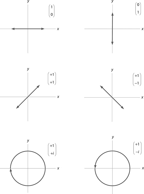
FIGURE 5.3 Various forms of polarization and their vector representation in Jones calculus.

The generalized polarization Jones matrix for linearly polarized light at an angle θ to the x-axis is given by

(\begin{matrix} a_{11} & a_{12} \\ a_{21} & a_{22} \end{matrix}) = (\begin{matrix} c o s^{2} θ & s i n θ c o s θ \\ s i n θ c o s θ & s i n^{2} θ \end{matrix}) (5.44)

$(\begin{matrix} a_{11} & a_{12} \\ a_{21} & a_{22} \end{matrix}) = (\begin{matrix} c o s^{2} θ & s i n θ c o s θ \\ s i n θ c o s θ & s i n^{2} θ \end{matrix}) (5.44)$

The right circular polarizer is described as

(\begin{matrix} a_{11} & a_{12} \\ a_{21} & a_{22} \end{matrix}) = \frac{1}{2} (\begin{matrix} 1 & - i \\ i & 1 \end{matrix}) (5.45)

$(\begin{matrix} a_{11} & a_{12} \\ a_{21} & a_{22} \end{matrix}) = \frac{1}{2} (\begin{matrix} 1 & - i \\ i & 1 \end{matrix}) (5.45)$

whereas the left circular polarizer is described as

(\begin{matrix} a_{11} & a_{12} \\ a_{21} & a_{22} \end{matrix}) = \frac{1}{2} (\begin{matrix} 1 & i \\ - i & 1 \end{matrix}) (5.46)

$(\begin{matrix} a_{11} & a_{12} \\ a_{21} & a_{22} \end{matrix}) = \frac{1}{2} (\begin{matrix} 1 & i \\ - i & 1 \end{matrix}) (5.46)$

The generalized rotation matrix for birefringent rotators is given by (Robson 1974)

(\begin{matrix} a_{11} & a_{12} \\ a_{21} & a_{22} \end{matrix}) = (\begin{matrix} c o s θ & s i n θ \\ - e^{i δ} s i n θ & e^{i δ} c o s θ \end{matrix}) (5.47)

$(\begin{matrix} a_{11} & a_{12} \\ a_{21} & a_{22} \end{matrix}) = (\begin{matrix} c o s θ & s i n θ \\ - e^{i δ} s i n θ & e^{i δ} c o s θ \end{matrix}) (5.47)$

where:

δ is the phase angle

α is the rotation angle about the z-axis

For a quarter-wave plate, δ = π/2, the rotation matrix becomes

(\begin{matrix} a_{11} & a_{12} \\ a_{21} & a_{22} \end{matrix}) = (\begin{matrix} c o s θ & s i n θ \\ - i s i n θ & i c o s θ \end{matrix}) (5.48)

$(\begin{matrix} a_{11} & a_{12} \\ a_{21} & a_{22} \end{matrix}) = (\begin{matrix} c o s θ & s i n θ \\ - i s i n θ & i c o s θ \end{matrix}) (5.48)$

5.4.1 Example

A laser beam linearly polarized in the x-direction is sent through an optical element that allows the transmission of y-polarization only, thus using Equations 5.36 and 5.42

(\begin{matrix} 0 & 0 \\ 0 & 1 \end{matrix}) (\begin{matrix} 1 \\ 0 \end{matrix}) = (\begin{matrix} 0 \\ 0 \end{matrix}) (5.49)

$(\begin{matrix} 0 & 0 \\ 0 & 1 \end{matrix}) (\begin{matrix} 1 \\ 0 \end{matrix}) = (\begin{matrix} 0 \\ 0 \end{matrix}) (5.49)$

so that no light is transmitted following the y-polarizer, as can be verified by a simple experiment.

5.5 Polarizing Prisms

There are two avenues to induce polarization using prisms. The first involves simple reflection as characterized by Fresnel’s equations and straightforward refraction. This approach is valid for windows, prisms, or multiple-prism arrays, made from homogeneous optical materials such as optical glass or fused silica. The second approach involves double refraction in crystalline transmission media exhibiting birefringence.

5.5.1 Transmission Efficiency in Multiple-Prism Arrays

Here, attention is focused on the polarization characteristics of multiple-prism arrays. First, we illustrate the use of transmission loss equations, which include the corresponding Fresnel coefficient, to evaluate the overall loss via an arbitrary number of incidence and exit surfaces. Second, an example involving a double-prism beam expander is given where the transmission losses, for both components of polarization, are calculated.

Images

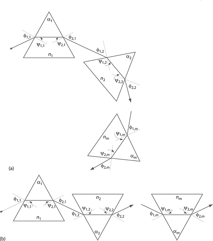
FIGURE 5.4 Generalized multiple-prism array in additive configuration (a) and compensating configuration (b). Depiction of multiple-prism arrays in this form was introduced by Duarte and Piper. (Data from Duarte F.J., and Piper, J.A., Am. J. Phys., 51, 1132–1134, 1983.)

For a generalized multiple-prism array, as shown in Figure 5.4, the cumulative reflection losses at the incidence surface of the mth prism are given by (Duarte et al. 1990)

L_{1, m} = L_{2, (m - 1)} + [1 - L_{2, (m - 1)}] ℛ_{1, m} (5.50)

$L_{1, m} = L_{2, (m - 1)} + [1 - L_{2, (m - 1)}] ℛ_{1, m} (5.50)$

whereas the losses at the mth exit surface are given by

L_{2, m} = L_{1, m} + (1 - L_{1, m}) ℛ_{2, m} (5.51)

$L_{2, m} = L_{1, m} + (1 - L_{1, m}) ℛ_{2, m} (5.51)$

where:

ℛ_1,m and ℛ_2,m are given by either ℛ_|| or ℛ_⊥

In practice, the optics is deployed so that the polarization of the propagation beam is parallel to the plane of incidence, meaning that the reflection coefficient is given by ℛ_||. It should be noted that these equations apply not just to prisms but also to optical wedges and any homogeneous optical element, with an input and exit surface, used in the transmission domain.

5.5.2 Induced Polarization in a Double-Prism Beam Expander

Polarization induction in multiple-prism beam expanders should be apparent once the reflectivity equations are combined with the transmission equations (5.50 and 5.51). In this section, this effect is made clear by considering the transmission efficiency, for both components of polarization, of a simple double-prism beam expander as illustrated in Figure 5.5. This beam expander is a modified version of one described by Duarte (2003) and consists of two identical prisms made of fused silica, with n = 1.4583 at λ ≈ 590 nm and an apex angle of 42.7098°. Both prisms are deployed to yield identical magnifications and for orthogonal beam exit. This implies that ϕ_1,1 = ϕ_1,2 = 81.55°, ψ_1,1 = ψ_1,2 = 42.7098°, ϕ_2,1 = ϕ_2,2 = 0°, and ψ_2,1 = ψ_2,2 = 0°.

Thus, for radiation polarized parallel to the plane of incidence,

\begin{matrix} L_{1, 1} = ℛ_{1, 1} = 0.3008 \\ L_{2, 1} = L_{1, 1} \\ L_{1, 2} = L_{2, 1} + (1 - L_{2, 1}) ℛ_{1, 2} = 0.5111 \\ L_{2, 2} = L_{1, 2} \end{matrix}

$\begin{matrix} L_{1, 1} = ℛ_{1, 1} = 0.3008 \\ L_{2, 1} = L_{1, 1} \\ L_{1, 2} = L_{2, 1} + (1 - L_{2, 1}) ℛ_{1, 2} = 0.5111 \\ L_{2, 2} = L_{1, 2} \end{matrix}$

whereas for radiation polarized perpendicular to the plane of incidence

L_{1, 1} = ℛ_{1, 1} = 0.5758

$L_{1, 1} = ℛ_{1, 1} = 0.5758$

Images

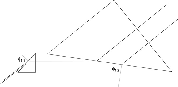
FIGURE 5.5 Double-prism expander as described in the text.

\begin{matrix} L_{2, 1} = L_{1, 1} \\ L_{1, 2} = L_{2, 1} + (1 - L_{2, 1}) ℛ_{1, 2} = 0.8200 \\ L_{2, 2} = L_{1, 2} \end{matrix}

$\begin{matrix} L_{2, 1} = L_{1, 1} \\ L_{1, 2} = L_{2, 1} + (1 - L_{2, 1}) ℛ_{1, 2} = 0.8200 \\ L_{2, 2} = L_{1, 2} \end{matrix}$

and also

\begin{matrix} k_{1, 1} = k_{1, 2} = 5.0005 \\ ℳ = k_{1, 1} k_{1, 2} = 25.0045 \end{matrix}

$\begin{matrix} k_{1, 1} = k_{1, 2} = 5.0005 \\ ℳ = k_{1, 1} k_{1, 2} = 25.0045 \end{matrix}$

Thus, for this particular beam expander, the cumulative reflection losses are 51.11% for light polarized parallel to the plane of incidence, whereas they increase to 82.00% for radiation polarized perpendicular to the plane of incidence. This example helps to illustrate the fact that multiple-prism beam expanders exhibit a clear polarization preference. It is easy to see that the addition of further stages of beam magnification leads to increased discrimination. When incorporated in frequency-selective dispersive laser cavities, these beam expanders contribute significantly toward the emission of laser emission polarized parallel to the plane of propagation where the polarization preference is reinforced by multiple-return passes.

See Chapter 4 for a generalized description of multiple-prism dispersion. Chapter 7 describes the use of multiple-prism arrays in laser oscillators.

5.6 Double-Refraction Polarizers

These are crystalline prism pairs that exploit the birefringence effect in crystals. In birefringent materials, the dielectric constant, ε, is different in each of the x, y, and z directions so that the propagation velocity is different in each direction:

v_{a} = c (ε_{x})^{- 1 / 2} (5.52)

$v_{a} = c (ε_{x})^{- 1 / 2} (5.52)$

v_{b} = c (ε_{y})^{- 1 / 2} (5.53)

$v_{b} = c (ε_{y})^{- 1 / 2} (5.53)$

v_{c} = c (ε_{z})^{- 1 / 2} (5.54)

$v_{c} = c (ε_{z})^{- 1 / 2} (5.54)$

Since polarization of a transmission medium is determined by the D vector, it is possible to describe the polarization characteristics in each direction. Further, it can be shown that there are two different velocities for the refracted radiation in any given direction (Born and Wolf 1999). As a consequence of the law of refraction, these two velocities lead to two different propagation paths in the crystal and give origin to the ordinary and extraordinary rays. In other words, the two velocities lead to double refraction.

Of particular interest in this class of polarizers are those known as the Nicol prism, the Rochon prism, the Glan–Foucault prism, the Glan–Thompson prism, and the Wollaston prism. According to Bennett and Bennett (1978), a Glan–Foucault prism pair is an air-spaced Glan–Thompson prism pair. In Glan-type polarizers, the extraordinary ray is transmitted from the first to the second prism in the propagation direction of the incident beam. However, the diagonal surfaces of the two prisms are predetermined to induce total internal reflection for the ordinary ray (see Figure 5.6). Glan-type polarizers are very useful since they can be oriented to discriminate in favor of either polarization component with negligible beam deviation. Normally, these polarizers are made of either quartz or calcite. Commercially available calcite Glan–Thompson polarizers with a useful aperture of 10 mm provide extinction ratios of ~5 × 10⁻⁵. It should be noted that Glan-type polarizers are used in straightforward propagation applications as well as intracavity elements. For instance, the tunable single-longitudinal-mode laser oscillator depicted in Figure 5.7 incorporates a Glan– Thompson polarizer as an output coupler. In this particular polarizer, the inner window is antireflection coated, whereas the outer window is coated for partial reflectivity to act as an output coupler mirror. The laser emission from multiple-prism grating oscillators is highly polarized parallel to the plane of incidence by the interaction of the intracavity flux with the multiple-prism expander and the grating. The function of the polarizer output coupler here is to provide further discrimination against unpolarized single-pass amplified spontaneous emission. These dispersive tunable laser oscillators yield extremely low levels of broadband amplified spontaneous emission measured to be in the 10⁻⁷ − 10⁻⁶ range (Duarte 1995, 1999).

Images

FIGURE 5.6 Generic Glan–Thompson polarizer. The beam polarized parallel to the plane of incidence is transmitted while the complementary component is deviated (drawing not to scale).

The Wollaston prism, illustrated in Figure 5.8, is usually fabricated of either crystalline quartz or calcite. These prisms are assembled from two matched and complementary right-angle prisms whose crystalline optical axes are oriented orthogonal to each other. These prisms are widely used as beam splitters of beams with orthogonal polarizations. The beam separation provided by calcite is significantly greater than that achievable with crystalline quartz. Also, for both materials, the beam separation is wavelength dependent.

Images

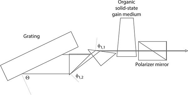
FIGURE 5.7 Solid-state MPL grating dye laser oscillator, yielding single-longitudinal-mode emission, incorporating a Glan–Thompson polarizer output coupler. The reflective coating is applied to the outer surface of the polarizer. (Reprinted from Opt. Commun., 117, Duarte, F.J., Solid-state dispersive dye laser oscillator: Very compact cavity, 480–484, Copyright 1995, with permission from Elsevier.)

Images

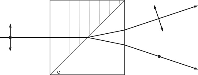
FIGURE 5.8 Generic Wollaston prism. The lines and circle represent the direction of the crystalline optical axis of the prism components (drawing not to scale).

The use of these prisms in quantum cryptography optical configurations is outlined in the work of Duarte (2014). In those optical configurations, a Wollaston prism is used after an electro-optical polarization rotator (such as a Pockels cell) to spatially separate photons corresponding to orthogonal polarizations. For a description of electro-optical polarization rotators, see the work of Saleh and Teich (1991).

5.7 Intensity Control of Laser Beams Using Polarization

A very simple, and yet powerful, technique to control and/or attenuate the intensity of linearly polarized laser beams involves the transmission of the laser beam through a prism pair such as a Glan–Thompson polarizer followed by rotation of the polarizer (Duarte 2001). The essence of this technique is illustrated in Figure 5.9. In this approach, for a ~100% laser beam polarized parallel to the plane of incidence, there is almost total transmission when the Glan–Thompson prism pair is oriented as in Figure 5.9a. As the prism pair is rotated about the axis of propagation, the intensity of the transmission decreases until it becomes zero once the angular displacement has reached π/2. With precision rotation of the prism pair, a scale of well-determined intensities can be easily obtained (Duarte 2001). This polarization attenuation technique has a number of applications including the generation of precise laser intensity scales for exposing instrumentation and laser printers used in imaging as discussed in Chapter 10 (Duarte 2001). Also, this technique has been successfully applied to laser cooling experiments to independently vary the intensity of the cooling and repumping lasers (Olivares et al. 2009).

Images

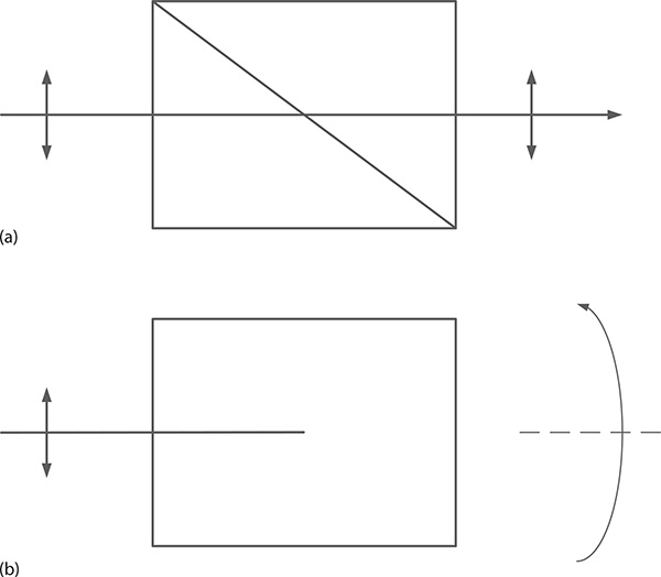
FIGURE 5.9 Attenuation of polarized laser beams using a Glan–Thompson polarizer: (a) polarizer set for ~100% transmission; (b) clockwise rotation of the polarizer, about the axis of propagation by π/2, yielding ~0% transmission. The amount of transmitted light can be varied continuously by rotating the polarizer in the 0 ≤ θ ≤ π/2 range. (Data from Duarte, F.J., Laser sensitometer using a multiple-prism beam expander and a polarizer. US Patent 6, 236, 461 B1, 2001.)

5.8 Polarization Rotators

Maximum transmission efficiency is always a goal in optical systems. If the polarization of a laser is mismatched to the polarization preference of the optics, then transmission efficiency will be poor. Furthermore, efficiency can be significantly improved if the polarization of a pump laser is matched to the polarization preference of the laser being excited (Duarte 1990). Although sometimes the efficiency can be improved, or even optimized, by the simple rotation of a laser, it is highly desirable and practical to have optical elements to perform this function. In this section, we shall consider two alternatives to perform such rotation: birefringent polarization rotators and prismatic rotators.

Images

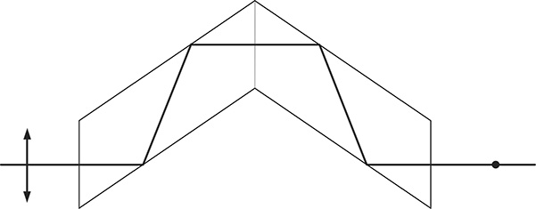
FIGURE 5.10 Side view of double Fresnel rhomb. Linearly polarized light is rotated by π/2 and exits with polarized orthogonally to the original polarization.

An additional alternative to rotate polarization are rhomboid configurations. For instance, double Fresnel rhomb (Figure 5.10), comprising two quarter-wave parallelepipeds, becomes a half-wave rhomb that rotates linearly polarized light by π/2. A commercially available Fresnel rhomb of this class, 10 mm wide and 53 mm long, offers a transmission efficiency close to 96% with broadband antireflection coatings. As indicated by Bennett and Bennett (1978), these achromatic rotators tend to offer a small useful aperture-to-length ratio and its achromaticity can be compromised by residual birefringence in the quartz. A description of the inner workings of Fresnel rhombs is offered by Born and Wolf (1999).

5.8.1 Birefringent Polarization Rotators

In birefringent uniaxial crystalline materials, the ordinary and extraordinary rays propagate at different velocities. The generalized matrix for birefringent rotators is given by Equation 5.47:

(\begin{matrix} a_{11} & a_{12} \\ a_{21} & a_{22} \end{matrix}) = (\begin{matrix} c o s θ & s i n θ \\ - e^{i δ} s i n θ & e^{i δ} c o s θ \end{matrix})

$(\begin{matrix} a_{11} & a_{12} \\ a_{21} & a_{22} \end{matrix}) = (\begin{matrix} c o s θ & s i n θ \\ - e^{i δ} s i n θ & e^{i δ} c o s θ \end{matrix})$

For a quarter-wave plate, δ = π/2, the phase term is e^iπ/2 = +i, and the rotation matrix becomes

(\begin{matrix} a_{11} & a_{12} \\ a_{21} & a_{22} \end{matrix}) = (\begin{matrix} c o s θ & s i n θ \\ - i s i n θ & i c o s θ \end{matrix}) (5.55)

$(\begin{matrix} a_{11} & a_{12} \\ a_{21} & a_{22} \end{matrix}) = (\begin{matrix} c o s θ & s i n θ \\ - i s i n θ & i c o s θ \end{matrix}) (5.55)$

For a half-wave plate, δ = π, and the phase term is eⁱ^π = −1. Thus, the rotation matrix becomes

(\begin{matrix} a_{11} & a_{12} \\ a_{21} & a_{22} \end{matrix}) = (\begin{matrix} c o s θ & s i n θ \\ s i n θ & - c o s θ \end{matrix}) (5.56)

$(\begin{matrix} a_{11} & a_{12} \\ a_{21} & a_{22} \end{matrix}) = (\begin{matrix} c o s θ & s i n θ \\ s i n θ & - c o s θ \end{matrix}) (5.56)$

From the experiment, we know that a half-wave plate causes a rotation of a linearly polarized beam by θ = π/2 so that Equation 5.56 reduces to

(\begin{matrix} a_{11} & a_{12} \\ a_{21} & a_{22} \end{matrix}) = (\begin{matrix} 0 & 1 \\ 1 & 0 \end{matrix}) (5.57)

$(\begin{matrix} a_{11} & a_{12} \\ a_{21} & a_{22} \end{matrix}) = (\begin{matrix} 0 & 1 \\ 1 & 0 \end{matrix}) (5.57)$

5.8.1.1 Example

Thus, if we send a beam polarized in the x-direction through a half-wave plate, the emerging beam polarization will be

(\begin{matrix} 0 & 1 \\ 1 & 0 \end{matrix}) (\begin{matrix} 1 \\ 0 \end{matrix}) = (\begin{matrix} 0 \\ 1 \end{matrix}) (5.58)

$(\begin{matrix} 0 & 1 \\ 1 & 0 \end{matrix}) (\begin{matrix} 1 \\ 0 \end{matrix}) = (\begin{matrix} 0 \\ 1 \end{matrix}) (5.58)$

which corresponds to a beam polarized in the y-direction as observed experimentally. In other words, polarization rotation by π/2 radians takes place.

5.8.2 Broadband Prismatic Polarization Rotators

An alternative to frequency-selective polarization rotators are prismatic rotators (Duarte 1989). These devices work at normal incidence and apply the principle of total internal reflection. The basic operation of polarization rotation, by π/2, due to total internal reflection is shown in Figure 5.11. This operation, however, reflects the beam into a direction that is orthogonal to the original propagation. Furthermore, the beam is not in the same plane. In order to achieve collinear polarization rotation, by π/2, the beam must be displaced upward and then be brought into alignment with the incident beam while conserving the polarization rotation achieved by the initial double reflection operation. A collinear prismatic polarization rotator, which performs this task using seven total internal reflections, is depicted in Figure 5.12. For high-power laser applications, this rotator is best assembled using a high-precision mechanical mount that allows air interfaces between the individual prisms. For a particular rotator, the useful aperture is about 10 mm and its physical length is 30 mm.

It should be noted that despite the apparent complexity of this collinear polarization rotator, the transmission efficiency is relatively high using antireflection coatings. In fact, using broadband (425–675 nm) antireflection coatings with a nominal loss of 0.5% per surface, the measured transmission efficiency becomes 94.7% at λ = 632.8 nm. The predicted transmission losses using

L_{r} = 1 - (1 - L)^{r} (5.59)

$L_{r} = 1 - (1 - L)^{r} (5.59)$

are 4.9%, with L = 0.5%, compared to a measured value of 5.3%. Equation 5.59 is derived combining Equations 5.50 and 5.51 for the special case of identical reflection losses. Here, r is the total number of reflection surfaces. For this particular col-linear rotator, r = 10. A further parameter of interest is the transmission fidelity of the rotator since it is also important to keep spatial distortions of the rotated beam to a minimum. The integrity of the beam due to transmission and rotation is quantified in Figure 5.13 where a very slight beam expansion of ~3.2% at full width at half maximum (FWHM) is evident (Duarte 1992).

Images

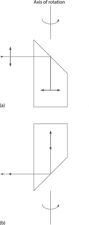
FIGURE 5.11 Basic prism operator for polarization rotation using two reflections. This can be composed of two 45° prisms adjoined π/2 to each other (note that it is also manufactured as one piece). (a) Side view of the rotator illustrating the basic rotation operation due to one reflection. The beam with the rotated polarization exists the prism into the plane of the figure. (b) The prism rotator is itself rotated anticlockwise by π/2 about the rotation axis (as indicated), thus providing an alternative perspective of the operation: the beam is now incident into the plane of the figure and it is reflected downward with its polarization rotated by π/2 relative to the original orientation. (Data from Duarte, F.J., Optical device for rotating the polarization of a light beam. US Patent 4, 822, 150, 1989.)

Images

FIGURE 5.12 Broadband collinear prism polarization rotator. (Data from Duarte, F.J., Optical device for rotating the polarization of a light beam. US Patent 4, 822, 150, 1989.)

5.8.2.1 Example

The π/2 prismatic polarization rotator just described rotates linearly x-polarized radiation into linearly y-polarized radiation and vice versa. Considering first the case of x →y and using the Jones matrix formalism, we can write

(\begin{matrix} a_{11} & a_{12} \\ a_{21} & a_{22} \end{matrix}) (\begin{matrix} 1 \\ 0 \end{matrix}) = (\begin{matrix} 1 a_{11} + 0 a_{12} \\ 1 a_{21} + 0 a_{22} \end{matrix}) = (\begin{matrix} 0 \\ 1 \end{matrix}) (5.60)

$(\begin{matrix} a_{11} & a_{12} \\ a_{21} & a_{22} \end{matrix}) (\begin{matrix} 1 \\ 0 \end{matrix}) = (\begin{matrix} 1 a_{11} + 0 a_{12} \\ 1 a_{21} + 0 a_{22} \end{matrix}) = (\begin{matrix} 0 \\ 1 \end{matrix}) (5.60)$

which means that a₁₁ = 0 and a₂₁ = 1. To find the other two components, we use the complementary rotation y → x that can be described as

(\begin{matrix} a_{11} & a_{12} \\ a_{21} & a_{22} \end{matrix}) (\begin{matrix} 0 \\ 1 \end{matrix}) = (\begin{matrix} 0 a_{11} + 1 a_{12} \\ 0 a_{21} + 1 a_{22} \end{matrix}) = (\begin{matrix} 1 \\ 0 \end{matrix}) (5.61)

$(\begin{matrix} a_{11} & a_{12} \\ a_{21} & a_{22} \end{matrix}) (\begin{matrix} 0 \\ 1 \end{matrix}) = (\begin{matrix} 0 a_{11} + 1 a_{12} \\ 0 a_{21} + 1 a_{22} \end{matrix}) = (\begin{matrix} 1 \\ 0 \end{matrix}) (5.61)$

which implies that a₁₂ 1 and a₂₂ 0. Thus, the Jones matrix for π/2 rotation, and that applies directly to the prismatic rotator described in Figure 5.12, becomes

R = (\begin{matrix} a_{11} & a_{12} \\ a_{21} & a_{22} \end{matrix}) = (\begin{matrix} 0 & 1 \\ 1 & 0 \end{matrix}) (5.62)

$R = (\begin{matrix} a_{11} & a_{12} \\ a_{21} & a_{22} \end{matrix}) = (\begin{matrix} 0 & 1 \\ 1 & 0 \end{matrix}) (5.62)$

Thus, we have again arrived to the π/2 rotation matrix (Equation 5.57) using simple linear algebra.

Images

FIGURE 5.13 Transmission fidelity of the broadband collinear polarization rotator: (a) intensity profile of incident beam, prior to rotation, and (b) intensity profile of transmitted beam with rotated polarization. (Reproduced from Duarte, F.J., Appl. Opt., 31, 3377–3378, 1992. With permission from the Optical Society.)

Problems

5.1. Design a single right-angle prism, made of fused silica, to expand a laser beam by a factor of 2 with orthogonal beam exit. Calculate ℛ_|| and ℛ_⊥. (Usen = 1.4583 at λ ≈ 590 nm.)

5.2. For a four-prism beam expander, with orthogonal beam exit, using fused silica prisms, calculate the overall beam magnification factor M for ϕ_1,1 = ϕ_1,2 = ϕ_1,3 = ϕ_1,3 = 70°. Also, calculate the overall transmission efficiency for a laser beam polarized parallel to the plane of incidence. (Use n = 1.4583 at λ ≈ 590 nm.)

5.3. Use Maxwell equations in the Gaussian system, for j = 0 and ρ = 0 case, to derive the wave equations:

\begin{matrix} \nabla^{2} E - (ε μ) c^{- 2} \frac{\partial^{2} E}{\partial t^{2}} = 0 \\ \nabla^{2} H - (ε μ) c^{- 2} \frac{\partial^{2} H}{\partial t^{2}} = 0 \end{matrix}

$\begin{matrix} \nabla^{2} E - (ε μ) c^{- 2} \frac{\partial^{2} E}{\partial t^{2}} = 0 \\ \nabla^{2} H - (ε μ) c^{- 2} \frac{\partial^{2} H}{\partial t^{2}} = 0 \end{matrix}$

5.4. If a linearly polarized beam in the x-direction is sent through a rotator plate represented by the matrix

(\begin{matrix} a_{11} & a_{12} \\ a_{21} & a_{22} \end{matrix}) = (\begin{matrix} 0 & 1 \\ - i & 0 \end{matrix})

$(\begin{matrix} a_{11} & a_{12} \\ a_{21} & a_{22} \end{matrix}) = (\begin{matrix} 0 & 1 \\ - i & 0 \end{matrix})$

What will be the polarization of the transmitted beam? What kind of plate would that be?

..................Content has been hidden....................

You can't read the all page of ebook, please click here login for view all page.

Table of Contents for
Chapter 5 Polarization

5

Polarization

5.1 Introduction

5.2 Maxwell Equations

5.3 Polarization and Reflection

5.3.1 Plane of Incidence

5.4 Jones Calculus

5.4.1 Example

5.5 Polarizing Prisms

5.5.1 Transmission Efficiency in Multiple-Prism Arrays

5.5.2 Induced Polarization in a Double-Prism Beam Expander

5.6 Double-Refraction Polarizers

5.7 Intensity Control of Laser Beams Using Polarization

5.8 Polarization Rotators

5.8.1 Birefringent Polarization Rotators

5.8.1.1 Example

5.8.2 Broadband Prismatic Polarization Rotators

5.8.2.1 Example

Problems

Table of Contents for Chapter 5 Polarization

Create new playlist

Sign In

Sign Up

Table of Contents for
Chapter 5 Polarization