Chapter 4 The Physics of Multiple- Prism Optics

Search in book...
Toggle Font Controls
Create new playlist

Name your new playlist

Playlist description (optional)
Sign In

Email address

Password

Forgot Password?

or

Continue with Facebook

Continue with Google
Sign Up

Full Name

Email address

Confirm Email Address

Password

or

Continue with Facebook

Continue with Google

Multiple-prism arrays were first introduced by Newton (1704) in his book Opticks. In this visionary volume, Newton reported on arrays of nearly isosceles prisms in additive and compensating configurations to control the propagation path and the dispersion of light. Further, he also illustrated slight beam expansion in a single isosceles prism. In his treatise, Newton does provide a written, qualitative, description of light dispersion in a sequence of prisms, thus providing the foundations for prismatic spectrometers and related instrumentation. In this chapter, a mathematical description of light dispersion in generalized multiple-prism arrays is given. Although the theory was originally developed to quantify the phenomenon of intracavity line-width narrowing in multiple-prism grating tunable laser oscillators (Duarte and Piper 1982), it is applicable beyond the domain of tunable lasers to optics in general. The theory considers single-pass as well as multiple-pass dispersion in generalized multiple-prism arrays and is useful to both linewidth narrowing and pulse compression. As a pedagogical tool, reduction of the generalized formulae to single-prism calculations is included in addition to a specific design of a particular practical high-magnification multiple-prism beam expander.

In order to facilitate the flow of information, and to maintain the focus on the physics, some of the mathematical steps involved in the derivations are not included. For further details, references to the original work are cited. The mathematical notation is consistent with the notation used in the original literature.

Besides a technical interest in quantifying multiple-prism arrays for laser, astronomical, and analytical instrumentation, the generalized multiple-prism dispersion theory is of interest from an intrinsic perspective. In the case of prismatic optics, the word dispersion really means the ranking or ordering of colors according to their wavelength. In other words, the phenomenon that is studied is the transition of white light, or broadband radiation, to highly ordered radiation according to its frequency. The multiple-prism dispersion theory enables the quantification of a transition from an initial state of entropy to a lower state of entropy—a transition that is rare in nature.

This chapter is a revised version of the original chapter published in the first edition of Tunable Laser Optics (Duarte 2003) and includes additional material on Amici prisms or compound prisms, generalized multiple-prism dispersion due to positive and negative refraction, and higher order phase derivatives for multiple-prism laser pulse compression.

4.2 Generalized Multiple-Prism Dispersion

Multiple-prism arrays are widely used in optics in a variety of applications such as (1) intracavity beam expanders in narrow-linewidth tunable laser oscillators, (2) extracavity beam expanders, (3) pulse compressors in ultrafast lasers, and (4) dispersive elements in spectrometers. Albeit multiple-prism arrays were first introduced by Newton (1704), a mathematical description of their dispersion had to wait a long time until their application as intracavity beam expanders in narrow-linewidth tunable lasers (Duarte and Piper 1982). Generalized multiple-prism arrays are depicted in Figure 4.1.

Images

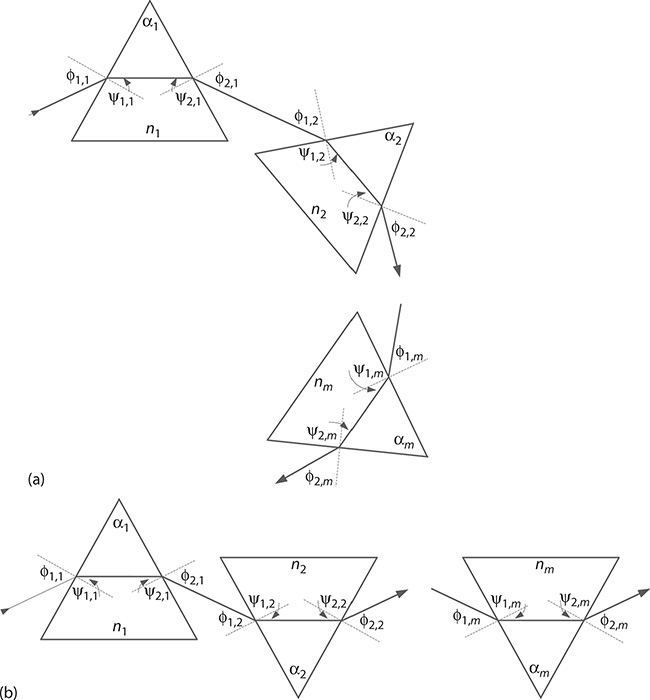
FIGURE 4.1 Generalized multiple-prism arrays: (a) Additive configuration; (b) compensating configuration. Depiction of these generalized prismatic configurations was introduced by Duarte and Piper. (Reproduced from Duarte, F.J., Quantum Optics for Engineers, CRC Press, New York, 2014. With permission from Taylor & Francis; Data from Duarte, F.J., and Piper, J.A., Am. J. Phys., 51, 1132–1134, 1983.)

Considering positive and negative refraction for the mth prism of the arrangements, the angular relations are given by (Duarte and Piper 1982; Duarte 2006)

ϕ 1, m + ϕ 2, m = ε m \pm α m (4.1)

$ϕ_{1, m} + ϕ_{2, m} = ε_{m} \pm α_{m} (4.1)$

ψ 1, m + ψ 2, m = α m (4.2)

$ψ_{1, m} + ψ_{2, m} = α_{m} (4.2)$

sin ϕ 1, m = \pm n m sin ψ 1, m (4.3)

$\sin ϕ_{1, m} = \pm n_{m} \sin ψ_{1, m} (4.3)$

sin ϕ 2, m = \pm n m sin ψ 2, m (4.4)

$\sin ϕ_{2, m} = \pm n_{m} \sin ψ_{2, m} (4.4)$

As illustrated in Figure 4.1, ϕ_1,m and ϕ_2,m are the angles of incidence and emergence, respectively, and ϕ_1,m and ϕ_2,m are the corresponding angles of refraction at the mth prism. In these equations, the positive sign (+) relates to positive refraction, whereas the negative sign (−) indicates negative refraction.

Differentiating Equations 4.3 and 4.4 and using

d ψ 1 , m d n = - d ψ 2 , m d n (4.5)

$\frac{d ψ_{1, m}}{d n} = - \frac{d ψ_{2, m}}{d n} (4.5)$

the single-pass dispersion following the mth prism is given by (Duarte and Piper 1982, 1983; Duarte 2006)

\nabla λ ϕ 2, m = \pm H 2, m \nabla λ n m \pm (k 1, m k 2, m) - 1 [H 1, m \nabla λ n m (\pm) \nabla λ ϕ 2, (m - 1)] (4.6)

$\nabla_{λ^{}} ϕ_{2, m} = \pm ℋ_{2, m} \nabla_{λ} n_{m} \pm (k_{1, m} k_{2, m})^{- 1} [ℋ_{1, m} \nabla_{λ} n_{m} (\pm) \nabla_{λ^{}} ϕ_{2, (m - 1)}] (4.6)$

where:

∇_λ = ∂/∂λ

and the following geometrical identities apply:

k 1, m = cos ψ 1 , m cos ϕ 1 , m (4.7)

$k_{1, m} = \frac{\cos ψ_{1, m}}{\cos ϕ_{1, m}} (4.7)$

k 2, m = cos ϕ 2 , m cos ψ 2 , m (4.8)

$k_{2, m} = \frac{\cos ϕ_{2, m}}{\cos ψ_{2, m}} (4.8)$

H 1, m = tan ϕ 1 , m n m (4.9)

$ℋ_{1, m} = \frac{\tan ϕ_{1, m}}{n_{m}} (4.9)$

H 2, m = tan ϕ 2 , m n m (4.10)

$ℋ_{2, m} = \frac{\tan ϕ_{2, m}}{n_{m}} (4.10)$

The k_1,m, and k_2,m, factors represent the physical beam expansion experienced at the mth prism by the incidence and emergence beams, respectively. In Equation 4.6, the signs in parentheses, that is, (±), refer to deployment in either a positive (+) or a compensating (−) configuration, while the simple ± indicates either positive or negative refraction (Duarte 2006).

The generalized single-pass dispersion equation indicates that the cumulative dispersion at the mth prism, namely, ∇_λϕ_2,m, is a function of the geometry of the mth prism, the position of the light beam relative to this prism, the material of this prism, and the cumulative dispersion up to the previous prism, ∇_λϕ_2,(m-1) (Duarte and Piper 1982, 1983). For completeness, it is useful to mention that the development of dispersive equations for both positive and negative refraction arises naturally from an interferometric perspective (Duarte 1993, 2006).

The generalized single-pass dispersion equation for positive refraction is

\nabla λ ϕ 2, m = H 2, m \nabla λ n m + (k 1, m k 2, m) - 1 [H 1, m \nabla λ n m \pm \nabla λ ϕ 2, (m - 1)] (4.11)

$\nabla_{λ^{}} ϕ_{2, m} = ℋ_{2, m} \nabla_{λ} n_{m} + (k_{1, m} k_{2, m})^{- 1} [ℋ_{1, m} \nabla_{λ} n_{m} \pm \nabla_{λ^{}} ϕ_{2, (m - 1)}] (4.11)$

For the special case of orthogonal beam exit, that is, ϕ_2,m = 0 and ψ_2,m = 0, we have ℋ_2,m = 0, k_2,m = 1 and Equation 4.11 reduces to

\nabla λ ϕ 2, m = (k 1, m) - 1 [H 1, m \nabla λ n m \pm \nabla λ ϕ 2, (m - 1)] (4.12)

$\nabla_{λ^{}} ϕ_{2, m} = (k_{1, m})^{- 1} [ℋ_{1, m} \nabla_{λ} n_{m} \pm \nabla_{λ^{}} ϕ_{2, (m - 1)}] (4.12)$

For an array of r identical isosceles or equilateral prisms deployed symmetrically in an additive configuration for positive refraction, so that ϕ_1,m = ϕ_2,m, the cumulative dispersion reduces to (Duarte 1990a)

\nabla λ ϕ 2, r = r \nabla λ ϕ 2, 1 (4.13)

$\nabla_{λ^{}} ϕ_{2, r} = r \nabla_{λ^{}} ϕ_{2, 1} (4.13)$

The generalized single-pass dispersion equation for positive refraction (Equation 4.11) can also be restated in a more practical and explicit notation (Duarte 1985, 1989, 1990a):

\nabla λ (ϕ 2, r = \sum r m = 1 (\pm 1) H 1, m (\prod r j = m k 1, j \prod r j = m k 2, j) - 1 \nabla λ n m + (M 1 M 2) - 1 \sum r m = 1 (\pm 1) H 2, m (\prod m j = 1 k 1, j \prod m j = 1 k 2, j) \nabla λ n m (4.14)

$\begin{matrix} \nabla_{λ^{(}} ϕ_{2, r} & = & \sum_{m = 1}^{r} (\pm 1) ℋ_{1, m} (\prod_{j = m}^{r} k_{1, j} \prod_{j = m}^{r} k_{2, j})^{- 1} \nabla_{λ} n_{m} \\ + (M_{1} M_{2})^{- 1} \sum_{m = 1}^{r} (\pm 1) ℋ_{2, m}^{} (\prod_{j = 1}^{m} k_{1, j} \prod_{j = 1}^{m} k_{2, j}) \nabla_{λ} n_{m} \end{matrix} (4.14)$

where:

M 1 = \prod j = 1 r k 1, j (4.15)

$M_{1} = \prod_{j = 1}^{r} k_{1, j} (4.15)$

and

M 2 = \prod j = 1 r k 2, j (4.16)

$M_{2} = \prod_{j = 1}^{r} k_{2, j} (4.16)$

are the respective beam expansion factors. For the important practical case of r right-angle prisms designed for orthogonal beam exit (i.e., ϕ_2,m = ψ_2,m = 0), Equation 4.14 reduces to

\nabla λ ϕ 2, r = \sum m = 1 r (\pm 1) H 1, m (\prod j = m r k 1, j) - 1 \nabla λ n m (4.17)

$\nabla_{λ^{}} ϕ_{2, r} = \sum_{m = 1}^{r} (\pm 1) ℋ_{1, m} (\prod_{j = m}^{r} k_{1, j})^{- 1} \nabla_{λ} n_{m} (4.17)$

If in addition the prisms have identical apex angles (α1=α2=α3=...=αm) $(α_{1} = α_{2} = α_{3} = ... = α_{m})$ and are configured to have the same angle of incidence (ϕ1,1= ϕ1,2= ϕ1,3=...= ϕ1,m) $(ϕ_{1, 1} = ϕ_{1, 2} = ϕ_{1, 3} = ... = ϕ_{1, m})$ , then Equation 4.17 can be written as (Duarte 1985)

\nabla λ ϕ 2, r = tan ψ 1, 1 \sum m = 1 r (\pm 1) (1 k 1 , m) m - 1 \nabla λ n m (4.18)

$\nabla_{λ^{}} ϕ_{2, r} = \tan ψ_{1, 1} \sum_{m = 1}^{r} (\pm 1) (\frac{1}{k_{1, m}})^{m - 1} \nabla_{λ} n_{m} (4.18)$

Further, if the angle of incidence for all prisms is Brewster’s angle, then the single-pass dispersion reduces to the elegant expression:

\nabla λ ϕ 2, r = \sum m = 1 r (\pm 1) (1 n m) m \nabla λ n m (4.19)

$\nabla_{λ^{}} ϕ_{2, r} = \sum_{m = 1}^{r} (\pm 1) (\frac{1}{n_{m}})^{m} \nabla_{λ} n_{m} (4.19)$

4.2.1 Double-Pass Generalized Multiple-Prism Dispersion

The evaluation of intracavity dispersion in tunable laser oscillators incorporating multiple-prism beam expanders requires the assessment of the double-pass, or return-pass, dispersion. The double-pass dispersion of multiple-prism beam expanders was derived by thinking of the return pass as a mirror image of the first light passage as illustrated in Figure 4.2. The return-pass dispersion corresponds to the dispersion experienced by the return light beam at the first prism. Thus, it is given by ∂tϕ1,m'/∂λ=∇λtϕ1,m' $\partial_{t ϕ_{1, m}'} / \partial λ = \nabla_{λ} t ϕ_{1, m}'$ , where the prime character indicates return pass (Duarte and Piper 1982, 1984):

\nabla λ ϕ 1, m' = H' 1, m \nabla λ n m + (k 1, m' k 2, m') [H' 2, m \nabla λ n m \pm \nabla λ ϕ 1, (m + 1)'] (4.20)

$\nabla_{λ^{}} ϕ_{1, m}' = ℋ_{1, m}^{'} \nabla_{λ} n_{m} + (k_{1, m}' k_{2, m}') [ℋ_{2, m}^{'} \nabla_{λ} n_{m} \pm \nabla_{λ^{}} ϕ_{1, (m + 1)}'] (4.20)$

where:

k 1, m' = cos ψ 1 , m ' cos ϕ 1 , m ' (4.21)

$k_{1, m}' = \frac{\cos ψ_{1, m}'}{\cos ϕ_{1, m}'} (4.21)$

k 2, m' = cos ϕ 2 , m ' cos ψ 2 , m, (4.22)

$k_{2, m}' = \frac{\cos ϕ_{2, m}'}{\cos ψ_{2, m}}, (4.22)$

H' 1, m = tan ϕ ' 1 , m n m (4.23)

$ℋ_{1, m}^{'} = \frac{\tan ϕ_{1, m}^{'}}{n_{m}} (4.23)$

H 2, m' = tan ϕ 2, m' ¯ ¯ ¯ ¯ ¯ ¯ ¯ ¯ ¯ ¯ ¯ ¯ ¯ (4.24)

$ℋ_{2, m}' =^{\underline{\tan ϕ_{2, m}'}} (4.24)$

Images

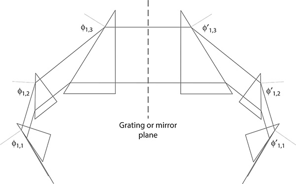
FIGURE 4.2 Multiple-prism beam expander geometry in additive configuration and its mirror image. A dispersive analysis through the multiple-prism array and its mirror image is equivalent to a double-pass, or return-pass, analysis. This type of description for multiple-prism grating assemblies was first introduced by Duarte and Piper. (Reproduced from Duarte, F.J., Quantum Optics for Engineers, CRC Press, New York, 2014. With permission from Taylor & Francis; Data from Duarte, F.J., and Piper, J.A., Opt. Commun., 43, 303–307, 1982.)

Here, ∇λtϕ1,(m+1)' $\nabla_{λ} t ϕ_{1, (m + 1)}'$ provides the cumulative single-pass multiple-prism dispersion and the dispersion of the diffraction grating, that is,

\nabla λ ϕ 1, (m + 1)' = (\nabla λ Θ G \pm \nabla λ ϕ 2, r) (4.25)

$\nabla_{λ^{}} ϕ_{1, (m + 1)}' = (\nabla_{λ} Θ_{G} \pm \nabla_{λ^{}} ϕ_{2, r}) (4.25)$

where:

∇_λΘ_G is the grating dispersion

If the grating is replaced by a mirror, then we simply have the prismatic contribution and

\nabla λ ϕ 1, (m + 1)' = \nabla λ ϕ 2, r (4.26)

$\nabla_{λ^{}} ϕ_{1, (m + 1)}' = \nabla_{λ^{}} ϕ_{2, r} (4.26)$

Defining ∇λtϕ1,m'=∇ΦP $\nabla_{λ} t ϕ_{1, m}' = \nabla Φ_{P}$ , where Φ stands for return pass and P for multiple prism, or a plurality of prisms, the explicit version of the generalized double-pass dispersion for a multiple-prism mirror system is given by (Duarte 1985, 1989)

\nabla λ Φ P = 2 M 1 M 2 \sum r m = 1 (\pm 1) H 1, m (\prod r j = m k 1, j \prod r j = m k 2, j) - 1 \nabla λ n m + 2 \sum r m = 1 (\pm 1) H 2, m (\prod m j = 1 k 1, j \prod m j = 1 k 2, j) \nabla λ n m (4.27)

$\begin{matrix} \nabla_{λ} Φ_{P} & = & 2 M_{1} M_{2} \sum_{m = 1}^{r} (\pm 1) ℋ_{1, m} (\prod_{j = m}^{r} k_{1, j} \prod_{j = m}^{r} k_{2, j})^{- 1} \nabla_{λ} n_{m} \\ + 2 \sum_{m = 1}^{r} (\pm 1) ℋ_{2, m}^{} (\prod_{j = 1}^{m} k_{1, j} \prod_{j = 1}^{m} k_{2, j}) \nabla_{λ} n_{m} \end{matrix} (4.27)$

For the case of r right-angle prisms designed for orthogonal beam exit (i.e., ϕ_2,m = ψ_2,m = 0), Equation 4.27 reduces to

\nabla λ Φ P = 2 M 1 \sum m = 1 r (\pm 1) H 1, m (\prod j = m r k 1, j) - 1 \nabla λ n m (4.28)

$\nabla_{λ} Φ_{P} = 2 M_{1} \sum_{m = 1}^{r} (\pm 1) ℋ_{1, m} (\prod_{j = m}^{r} k_{1, j})^{- 1} \nabla_{λ} n_{m} (4.28)$

which can also be expressed as (Duarte 1985)

\nabla λ Φ P = 2 \sum m = 1 r (\pm 1) (\prod j = 1 m k 1, j) tan ψ 1, m \nabla λ n m (4.29)

$\nabla_{λ} Φ_{P} = 2 \sum_{m = 1}^{r} (\pm 1) (\prod_{j = 1}^{m} k_{1, j}) \tan ψ_{1, m} \nabla_{λ} n_{m} (4.29)$

If the angle of incidence for all prisms in the array is made equal to the Brewster angle, this equation simplifies further to (Duarte 1990a)

\nabla λ Φ P = 2 \sum m = 1 r (\pm 1) (n m) m - 1 \nabla λ n m (4.30)

$\nabla_{λ} Φ_{P} = 2 \sum_{m = 1}^{r} (\pm 1) (n_{m})^{m - 1} \nabla_{λ} n_{m} (4.30)$

Images

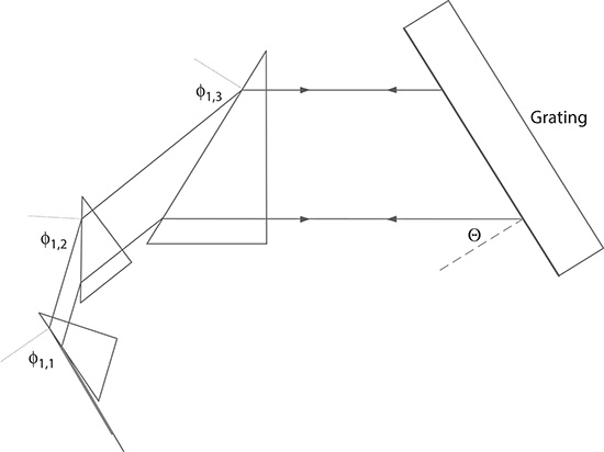
FIGURE 4.3 Additional perspective on the multiple-prism grating assembly used to perform the dispersive multiple-return pass analysis as explained by Duarte and Piper. The multiple-prism configuration can be either additive or compensating and can be composed of any number of prisms. (Data from Duarte, F.J., and Piper, J.A., Opt. Commun., 43, 303–307, 1982.)

4.2.2 Multiple Return-Pass Generalized Multiple-Prism Dispersion

Here we consider a multiple-prism grating or multiple-prism mirror assembly as illustrated in Figures 4.2 and 4.3. The light beam enters the first prism of the array, it is then expanded, and it is either diffracted back or reflected back into the multiple-prism array. In a dispersive laser oscillator, this process goes forth and back many times, thus giving rise to the concept of intracavity double pass or intracavity return pass. For the first return pass toward the first prism in the array, the dispersion is given by

\nabla λ ϕ 2, m = H 2, m \nabla λ n m + (k 1, m k 2, m) - 1 [H 1, m \nabla λ n m \pm \nabla λ ϕ 2, (m - 1)]

$\nabla_{λ^{}} ϕ_{2, m} = ℋ_{2, m} \nabla_{λ} n_{m} + (k_{1, m} k_{2, m})^{- 1} [ℋ_{1, m} \nabla_{λ} n_{m} \pm \nabla_{λ^{}} ϕ_{2, (m - 1)}]$

If N denotes the number of passes toward the grating or reflecting element and 2N denotes the number of return passes toward the first prism in the sequence, we have (Duarte and Piper 1984)

(\nabla λ ϕ 2, m) N = H 2, m \nabla λ n m + (k 1, m k 2, m) - 1 {H 1, m \nabla λ n m \pm [\nabla λ ϕ 2, (m - 1)] N} (4.31)

$(\nabla_{λ^{}} ϕ_{2, m})_{N} = ℋ_{2, m} \nabla_{λ} n_{m} + (k_{1, m} k_{2, m})^{- 1} {ℋ_{1, m} \nabla_{λ} n_{m} \pm [\nabla_{λ^{}} ϕ_{2, (m - 1)}]_{N}} (4.31)$

and

(\nabla λ ϕ 1, m') 2 N = H r 1, m \nabla λ n m + (k 1, m' k 2, m') {H f 2, m' \nabla λ n m \pm [\nabla λ ϕ 1, (m + 1)'] 2 N} (4.32)

$(\nabla_{λ^{}} ϕ_{1, m}')_{2 N} = ℋ^{r_{1, m}} \nabla_{λ} n_{m} + (k_{1, m}' k_{2, m}') {H f_{2, m}' \nabla_{λ} n_{m} \pm [\nabla_{λ^{}} ϕ_{1, (m + 1)}']_{2 N}} (4.32)$

For the first prism of the array, [∇_λϕ_2,(m-1)]_N (with N = 3, 5, 7, …) in Equation 4.31 is replaced by (∇_λϕ′_1,1)_2N (with N = 1, 2, 3, …). Likewise for the last prism of the assembly, [∇_λϕ′_1,(m+1)]_2N (with N = 1, 3, 5, …) in Equation 4.32 is replaced by [∇_λΘ_G + (∇_λϕ_2,r)_N] (with N = 1, 2, 3, …). In the case of the grating being replaced by a mirror, this expression becomes simply (∇_λϕ_2,r)_N) (with N = 1, 3, 5, …). Thus, the multiple return-pass dispersion for a multiple-prism grating assembly is given by (Duarte and Piper 1984)

(\nabla λ θ) R = (R M \nabla λ Θ G + R \nabla λ Φ P) (4.33)

$(\nabla_{λ} θ)_{R} = (R M \nabla_{λ} Θ_{G} + R \nabla_{λ} Φ_{P}) (4.33)$

where:

R is the number of return passes

M is the overall beam magnification of the multiple-prism beam expander

This equation illustrates the very important fact that in the return-pass dispersion of a multiple-prism grating assembly, the dispersion of a grating is multiplied by the factor RM. Once again, if the grating is replaced by a mirror, that is, ∇_λΘ_G = 0, the dispersion reduces to

(\nabla λ θ) R = R \nabla λ Φ P (4.34)

$(\nabla_{λ} θ)_{R} = R \nabla_{λ} Φ_{P} (4.34)$

which implies that the multiple-prism intracavity dispersion increases linearly as a function of R. In practice, the quantity R has a limit imposed by experimental conditions and is usually R ≈ 3 for pulsed high-power narrow-linewidth tunable organic lasers emitting in the nanosecond regime (Duarte and Piper 1984; Duarte 2001a) (see Section 4.3.1).

4.2.3 Single-Prism Equations

Using Equation 4.11 for m = 1 yields

\nabla λ ϕ 2, m = H \cap 2, 1 \nabla λ n 1 + (k 1, 1 k 2, 1) - 1 (H 1, m \nabla λ n 1) (4.35)

$\nabla_{λ^{}} ϕ_{2, m} = ℋ_{2, 1}^{\cap} \nabla_{λ} n_{1} + (k_{1, 1} k_{2, 1})^{- 1} (ℋ_{1, m} \nabla_{λ} n_{1}) (4.35)$

which can also be expressed as (Duarte 1990a)

\nabla λ ϕ 2, 1 = (sin ψ 2 , 1 cos ϕ 2 , 1) \nabla λ n 1 + (cos ψ 2 , 1 cos ϕ 2 , 1) tan ψ 1, 1 \nabla λ n 1 (4.36)

$\nabla_{λ^{}} ϕ_{2, 1} = (\frac{\sin ψ_{2, 1}}{\cos ϕ_{2, 1}}) \nabla_{λ} n_{1} + (\frac{\cos ψ_{2, 1}}{\cos ϕ_{2, 1}}) \tan ψ_{1, 1} \nabla_{λ} n_{1} (4.36)$

Division by ∇_λn yields the result given for ∇_nϕ_2,1 by Born and Wolf (1999). For orthogonal beam exit ( ϕ2,1≈ψ2,1≈0) $(ϕ_{2, 1} \approx ψ_{2, 1} \approx 0)$ , Equation 4.36 simplifies to

\nabla λ ϕ 2, 1 \approx tan ψ 1, 1 \nabla λ n (4.37)

$\nabla_{λ^{}} ϕ_{2, 1} \approx \tan ψ_{1, 1} \nabla_{λ} n (4.37)$

which is the result given by Wyatt (1978). For a single prism designed for orthogonal beam exit and deployed at Brewster’s angle of incidence, Equation 4.19 becomes

\nabla λ ϕ 2, 1 = (1 n) \nabla λ n (4.38)

$\nabla_{λ^{}} ϕ_{2, 1} = (\frac{1}{n}) \nabla_{λ} n (4.38)$

a result that also follows from Equation 4.37.

For a double-pass analysis, for m = 1, Equation 4.32 becomes

\nabla λ ϕ 1, 1' = H' 1, 1 \nabla λ n 1 + (k 1, 1' k 2, 1') (H' 2, 1 \nabla λ n 1 \pm \nabla λ ϕ 2, 1) (4.39)

$\nabla_{λ^{}} ϕ_{1, 1}' = ℋ_{1, 1}^{'} \nabla_{λ} n_{1} + (k_{1, 1}' k_{2, 1}') (ℋ_{2, 1}^{'} \nabla_{λ} n_{1} \pm \nabla_{λ^{}} ϕ_{2, 1}) (4.39)$

which for orthogonal beam exit reduces to

\nabla λ Φ P = 2 (k 1, 1 tan ψ 1, 1) \nabla λ n (4.40)

$\nabla_{λ} Φ_{P} = 2 (k_{1, 1} \tan ψ_{1, 1}) \nabla_{λ} n (4.40)$

For incidence at the Brewster angle, this equation simplifies further to

\nabla λ Φ P = 2 \nabla λ n (4.41)

$\nabla_{λ} Φ_{P} = 2 \nabla_{λ} n (4.41)$

Reduction from Equation 4.40 to 4.41 implies that at the Brewster angle of incidence, the beam magnification

tan ψ 1, 1 = 1 n (4.42)

$\tan ψ_{1, 1} = \frac{1}{n} (4.42)$

and

tan ψ 1, 1 = 1 ¯ (4.43)

$\tan ψ_{1, 1} = \underline{1} (4.43)$

4.3 Multiple-Prism Dispersion Linewidth Narrowing

The cavity linewidth equation is derived, in Chapter 3, from interferometric principles as (Duarte 1992)

Δ λ = Δ θ (\nabla λ θ) - 1 (4.44)

$Δ λ = Δ θ (\nabla_{λ} θ)^{- 1} (4.44)$

where:

Δθ is the beam divergence

∇_λθ is the overall intracavity dispersion

The message from this equation is that for narrow-linewidth emission we need to minimize the beam divergence and to increase the intracavity dispersion. The multiple-return-pass cavity linewidth for dispersive oscillator configurations, as illustrated in Figures 4.4 and 4.5, is given by (Duarte 2001b)

Δ λ = Δ θ R (M R \nabla λ Θ G + R \nabla λ Φ P) - 1 (4.45)

$Δ λ = Δ θ_{R} (M R \nabla_{λ} Θ_{G} + R \nabla_{λ} Φ_{P})^{- 1} (4.45)$

and the multiple-return-pass beam divergence (see Chapter 6) is given by

Δ θ R = λ π w [1 + (L R J B R) 2 + (A R L R B R) 2] 1 / 2 (4.46)

$Δ θ_{R} = \frac{λ}{π w} [1 + (\frac{L_{R J}}{B_{R}})^{2} + (\frac{A_{R} L_{R}}{B_{R}})^{2}]^{1 / 2} (4.46)$

where:

w is the beam waist

L_ℛ(πw²/λ) is the Rayleigh length

A_R and B_R are multiple-pass propagation matrix coefficients

For an optimized multiple-prism grating laser oscillator, Δθ_R approaches its diffraction limit following a few return passes.

4.3.1 Mechanics of Linewidth Narrowing in Optically Pumped Pulsed Laser Oscillators

The factor R in the multiple-return-pass linewidth equation is related to the total intracavity transit time from the beginning of the excitation pulse to the onset of laser oscillation. Thus, R is determined experimentally by measuring the time delay δτ between the leading edge of the pump pulse and the leading edge of the laser emission pulse. This perspective is consistent with the mechanics of recording single-pulse interferograms, which provide the laser linewidth at the early stages of oscillation that is broader than at subsequent times of emission. That is, although the linewidth narrowing continues throughout the duration of the laser emission, the time-integrated recording process, using photographic means for instance, yields information as broad as that recorded at the onset of the laser oscillation. Once δτ has been measured, the number return intracavity passes is given by

R = δ τ Δ t (4.47)

$R = \frac{δ τ}{Δ t} (4.47)$

Images

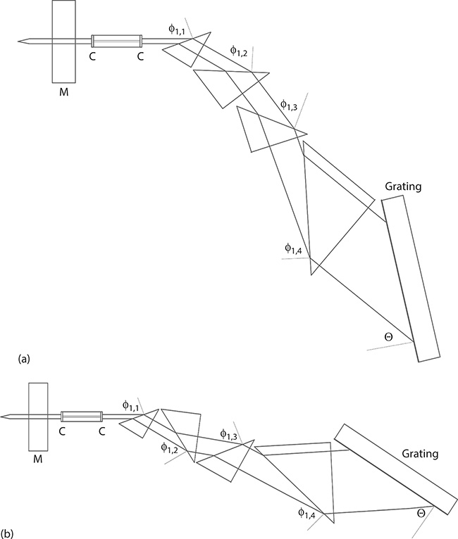
FIGURE 4.4 (a) MPL grating semiconductor laser oscillators incorporating a (+, +, +, -) compensating multiple-prism configuration (a) and a (+, -, +, -) compensating multiple-prism configuration (b). (Reproduced from Duarte, F.J., Tunable Laser Applications, 2nd edn., Chapter 5, CRC Press, New York, 2009. With permission from Taylor & Francis.)

where:

Δt is the time taken by the emission to cover twice the cavity length or Δt = 2L/c so that

R = δ τ (c 2 L) (4.48)

$R = δ τ (\frac{c}{2 L}) (4.48)$

In sum, from the beginning of the pulsed laser excitation, the R factor contributes to reduce both the beam divergence and the laser linewidth. As indicated by Equation 4.46, the beam divergence can only decrease toward its diffraction limit, whereas the laser linewidth decreases linearly as a function of R. In turn, R is a finite number that can be as low as R ≈ 3 for high-power short-pulse excitation. It is also necessary to remember that Equation 4.45 is the dispersive cavity linewidth equation, that is, it quantifies the ability of a dispersive oscillator cavity to narrow the frequency transmission window of the cavity. Once the dispersion linewidth limits emission to a single longitudinal mode, the actual linewidth of that mode is determined by the dynamics of the laser. For further information on this subject, the reader should refer to Duarte and Piper (1984) and Duarte (2001b).

Images

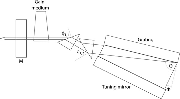
FIGURE 4.5 HMPGI grating solid-state organic laser oscillator incorporating a compensating (+, -) double-prism configuration. (Reprinted from Opt. Laser Technol., 29, Duarte, F.J., Multiple-prism near-grazing-incidence grating solid-state dye-laser oscillator, 513–519, Copyright 1997, with permission from Elsevier.)

4.3.2 Design of Zero-Dispersion Multiple-Prism Beam Expanders

In practice, the dispersion of the grating multiplied by the beam expansion, that is, M(∇_λΘ_G), amply dominates the overall intracavity dispersion. Thus, it is desirable to remove the dispersion component originating from the multiple-prism beam expander so that

Δ λ \approx Δ θ R (M R \nabla λ Θ G) - 1 (4.49)

$Δ λ \approx Δ θ_{R} (M R \nabla_{λ} Θ_{G})^{- 1} (4.49)$

At this stage, we go back to Equation 4.29 and set the requirement ∇_λΘ_P = 0 so that (Duarte 1985)

\nabla λ Φ P = 2 \sum m = 1 r (\pm 1) (\prod j = 1 m k 1, j) tan ψ 1, m \nabla λ n m = 0

$\nabla_{λ} Φ_{P} = 2 \sum_{m = 1}^{r} (\pm 1) (\prod_{j = 1}^{m} k_{1, j}) \tan ψ_{1, m} \nabla_{λ} n_{m} = 0$

For a double-prism expander yielding zero dispersion,

(k 1, 1) tan ψ 1, 1 = (k 1, 1) k 1, 2 tan ψ 1, 2 (4.50)

$(k_{1, 1}) \tan ψ_{1, 1} = (k_{1, 1}) k_{1, 2} \tan ψ_{1, 2} (4.50)$

For a three-prism expander yielding zero dispersion,

(k 1, 1 + k 1, 1 k 1, 2) tan ψ 1, 1 = (k 1, 1 k 1, 2) k 1, 3 tan ψ 1, 3 (4.51)

$(k_{1, 1} + k_{1, 1} k_{1, 2}) \tan ψ_{1, 1} = (k_{1, 1} k_{1, 2}) k_{1, 3} \tan ψ_{1, 3} (4.51)$

For a four-prism expander yielding zero dispersion,

(k 1, 1 + k 1, 1 k 1, 2 + k 1, 1 k 1, 2 k 1, 3) tan ψ 1, 1 = (k 1, 1 k 1, 2 k 1, 3) k 1, 4 tan ψ 1, 4 (4.52)

$(k_{1, 1} + k_{1, 1} k_{1, 2} + k_{1, 1} k_{1, 2} k_{1, 3}) \tan ψ_{1, 1} = (k_{1, 1} k_{1, 2} k_{1, 3}) k_{1, 4} \tan ψ_{1, 4} (4.52)$

For a five-prism expander yielding zero dispersion,

(k 1, 1 + k 1, 1 k 1, 2 + k 1, 1 k 1, 2 k 1, 3 + k 1, 1 k 1, 2 k 1, 3 k 1, 4) tan ψ 1, 1 = (k 1, 1 k 1, 2 k 1, 3 k 1, 4) k 1, 5 tan ψ 1, 5 (4.53)

$(k_{1, 1} + k_{1, 1} k_{1, 2} + k_{1, 1} k_{1, 2} k_{1, 3} + k_{1, 1} k_{1, 2} k_{1, 3} k_{1, 4}) \tan ψ_{1, 1} = (k_{1, 1} k_{1, 2} k_{1, 3} k_{1, 4}) k_{1, 5} \tan ψ_{1, 5} (4.53)$

The beauty of these zero-dispersion multiple-prism configurations is that the multiple-prism expander contributes to greatly augment the intracavity dispersion, while the tuning characteristics of the laser are exclusively determined by the diffraction grating.

4.3.2.1 Example

To illustrate the design of a quasi-achromatic multiple-prism beam expander, a case of practical interest, with M ≈ 100, and a four-prism expander deployed in a compensating configuration, similar to that outlined in Figure 4.4a, is considered. The compensating configuration selected is (+, +, +, -); that is, the additive dispersion of the first three prisms is subtracted by the fourth prism, thus yielding zero overall dispersion. Multiple-prism beam expanders deployed intracavity in tunable lasers employ right-angle prisms designed for orthogonal beam exit, that is, ϕ_2,m ≈ ψ_2,m ≈ 0. Thus, we apply Equation 4.52:

(k 1, 1 + k 1, 1 k 1, 2 + k 1, 1 k 1, 2 k 1, 3) tan ψ 1, 1 = (k 1, 1 k 1, 2 k 1, 3) k 1, 4 tan ψ 1, 4

$(k_{1, 1} + k_{1, 1} k_{1, 2} + k_{1, 1} k_{1, 2} k_{1, 3}) \tan ψ_{1, 1} = (k_{1, 1} k_{1, 2} k_{1, 3}) k_{1, 4} \tan ψ_{1, 4}$

If the first three prisms are identical, then we have

tan ψ 1, 1 = tan ψ 1, 2 = tan ψ 1, 3 (4.54)

$\tan ψ_{1, 1} = \tan ψ_{1, 2} = \tan ψ_{1, 3} (4.54)$

A particular wavelength of interest in tunable lasers is λ = 590 nm. At this wavelength, for a material such as optical crown glass, n = 1.5167. For M ≈ 100, we select

k 1, 1 k 1, 2 k 1, 3 = 64

$k_{1, 1} k_{1, 2} k_{1, 3} = 64$

so that

k 1, 1 = k 1, 2 = k 1, 3 = 4

$k_{1, 1} = k_{1, 2} = k_{1, 3} = 4$

This means that for the first three prisms

ϕ 1, 1 = ϕ 1, 2 = ϕ 1, 3 = 79.0 1 o

$ϕ_{1, 1} = ϕ_{1, 2} = ϕ_{1, 3} = 79.0 1^{o}$

and

ψ 1, 1 = ψ 1, 2 = ψ 1, 3 = 40.3 3 o

$ψ_{1, 1} = ψ_{1, 2} = ψ_{1, 3} = 40.3 3^{o}$

which also becomes the apex angle of the first three prisms. Using Equation 4.52, it is found that for the fourth prism, ϕ_1,4 = 59.39°, ψ_1,4 = 34.57°, and k_1,4 = 1.62. This yields an overall beam magnification factor of M = 64 × 1.62 ≈ 103.68. Normally, the beam waist w in a well-designed high-power multiple-prism grating laser oscillator is about 100 μm. This means that the expanded beam at the exit surface of the fourth prism is 2wM ≈ 20.7 mm. Thus, this particular multiple-prism beam expander can be composed of three small prisms with a hypotenuse of 17 mm, albeit the first two can be even smaller. The larger fourth prism requires a hypotenuse of 27 mm. The thickness of all prisms can be 10 mm. The surfaces of these prisms are usually polished to yield a surface flatness of λ/4 or better.

4.3.2.2 Example

Optimized compact high-power solid-state multiple-prism laser oscillators have been demonstrated to yield single-longitudinal-mode oscillation at Δν ≈ 350 MHz, at pulses Δt ≈ 3 ns, near the limit allowed by Heisenberg’s uncertainty principle (Duarte 1999). The oscillator, illustrated in Figure 4.6, requires the use of a small fused silica double-prism beam expander with M ≈ 42 and ϕ_2,m ≈ ψ_2,m ≈ 0 at λ = 590 nm. Thus we use Equation 4.29 or 4.50 to obtain (Duarte 2000)

tan ψ 1, 1 = k 1, 2 tan ψ 1, 2 (4.55)

$\tan ψ_{1, 1} = k_{1, 2} \tan ψ_{1, 2} (4.55)$

For n = 1.4583 and ϕ_1,1 = 88.60°, we get ψ_1,1 = 43.28° and k_1,1 ≈ 29.80. With these initial parameters, Equation 4.55 yields for the second prism ϕ_1,2 ≈ 53.93°, ψ_1,2 = 33.66° and k_1,2 ≈ 1.41. Therefore, the overall intracavity beam expansion becomes

M = k 1, 1 k 1, 2 \approx 42.13

$M = k_{1, 1} k_{1, 2} \approx 42.13$

Images

FIGURE 4.6 Optimized multiple-prism grating tunable organic laser oscillator incorporating a compensating (+, -) double-prism configuration. This oscillator demonstrated single-transverse-mode beam characteristics and single-longitudinal-mode emission at Δν ≈ 350 MHz and Δt ≈ 3 ns. (Reproduced from Duarte, F.J., Appl. Opt., 38, 6347–6349, 1999. With permission from the Optical Society.)

For a beam waist of w = 100 μm, this implies 2wM ≈ 8.43 mm. These dimensions require the first prism to have a hypotenuse of ~8 mm and the second prism a hypotenuse of ~10 mm. In this particular oscillator, this intracavity beam expansion is used to illuminate a 3300 lines/mm grating deployed at an angle of incidence ~77° in Littrow configuration (Duarte 1999).

Shay and Duarte (2009) describe the design of a zero-dispersion five-prism beam expander for fused silica at λ = 1550 nm (n = 1.44402), yielding an overall beam expansion of M ≈ 987.

4.4 Dispersion of Amici, or Compound, Prisms

Amici prisms, direct-vision prisms, and compound prisms are terms that refer to multiple-prism assemblies designed not to deviate the light beam. In this regard, such prisms are essentially multiple-prism arrays where the prisms are deployed, in compensating configurations, right next to each other without space in between. One of the main applications of Amici prisms is in the field of astronomy for the correction of atmospheric dispersion in adaptive optics systems for very large telescopes (Wynne 1997). The description of the dispersion calculation of Amici prisms given here follows a review given by Duarte (2013). The expression applied here is the single-pass generalized multiple-prism dispersion equation for positive refraction, that is, Equation 4.11:

\nabla λ ϕ 2, m = H 2, m \nabla λ n m + (k 1, m k 2, m) - 1 [H 1, m \nabla λ n m \pm \nabla λ ϕ 2, (m - 1)]

$\nabla_{λ^{}} ϕ_{2, m} = ℋ_{2, m} \nabla_{λ} n_{m} + (k_{1, m} k_{2, m})^{- 1} [ℋ_{1, m} \nabla_{λ} n_{m} \pm \nabla_{λ^{}} ϕ_{2, (m - 1)}]$

For a single prism (m = 1), as illustrated in Figure 4.7, this equation reduces to Equation 4.35:

\nabla λ ϕ 2, 1 = H 2, 1 \nabla λ n 1 + (k 1, 1 k 2, 1) - 1 (H 1, m \nabla λ n 1)

$\nabla_{λ^{}} ϕ_{2, 1} = ℋ_{2, 1} \nabla_{λ} n_{1} + (k_{1, 1} k_{2, 1})^{- 1} (ℋ_{1, m} \nabla_{λ} n_{1})$

Images

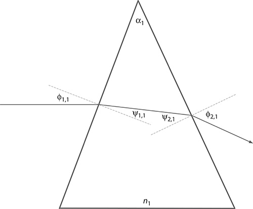
FIGURE 4.7 Single dispersive prism, made of fused silica, with a negative dispersion of ∇_λϕ_2,1 ≈ −0.0386 for the D₂ line of sodium at λ = 588.9963 nm. The calculations indicate a severe beam deviation.

For a double-prism configuration (m = 2) in a compensating mode, as illustrated in Figure 4.8, the dispersion equation becomes

\nabla λ ϕ 2, 2 = H 2, 2 \nabla λ n m + (k 1, 2 k 2, 2) - 1 (H 1, 2 \nabla λ n m \pm \nabla λ ϕ 2, 1) (4.56)

$\nabla_{λ^{}} ϕ_{2, 2} = ℋ_{2, 2} \nabla_{λ} n_{m} + (k_{1, 2} k_{2, 2})^{- 1} (ℋ_{1, 2} \nabla_{λ} n_{m} \pm \nabla_{λ^{}} ϕ_{2, 1}) (4.56)$

and for a three-prism (m = 3) compensating configuration, as illustrated in Figure 4.9, the dispersion equation becomes

\nabla λ ϕ 2, 3 = H 2, 3 \nabla λ n m + (k 1, 3 k 2, 3) - 1 (H 1, 3 \nabla λ n m \pm \nabla λ ϕ 2, 2) (4.57)

$\nabla_{λ^{}} ϕ_{2, 3} = ℋ_{2, 3} \nabla_{λ} n_{m} + (k_{1, 3} k_{2, 3})^{- 1} (ℋ_{1, 3} \nabla_{λ} n_{m} \pm \nabla_{λ^{}} ϕ_{2, 2}) (4.57)$

thus explicitly illustrating the iterative nature of the generalized multiple-prism equations.

Images

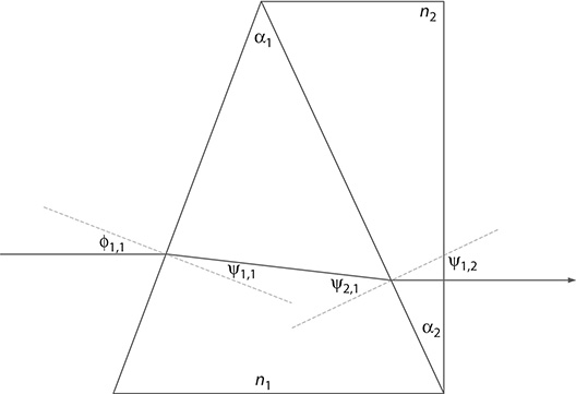
FIGURE 4.8 Double-prism Amici configuration comprising a fused silica prism and a higher diffractive index Schott SF10 prism. Here, ∇_λϕ_2,2 ≈ -0.0330 at λ = 588.9963 nm and the exit beam is in the same direction, albeit still displaced, as the incident beam. (Drawing not to scale.)

Images

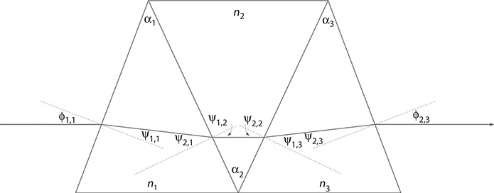
FIGURE 4.9 Three-prism Amici, direct-vision, configuration. The first and third prisms are made of fused silica (n₁ = n₃ = 1.458413), whereas the second prism, positioned at the center of the configuration, is made of Schott SF10 (n₂ = 1.728093). As explained in the text, this compound prism is formed by unfolding the double-prism configuration shown in Figure 4.8. Here, the overall dispersion is ∇_λϕ_2,3 ≈ +0.0720 at λ = 588.9963 nm, and the exit beam is collinear with the incident beam as discussed in the text. (Drawing not to scale.)

4.4.1 Example

Here, the design and evaluation of dispersion for a two-prism and a three-prism Amici configuration is demonstrated following the example given by Duarte (2013). Selecting a fused silica prism (n₁ = 1.458413 at λ = 588.9963 nm, also known as the sodium D₂ line), as the first dispersive stage, with the following angular dimensions α₁ = 45°, ϕ_1,1 = 20.66°, ψ_1,1 = 14.00°, ψ_2,1 = 31.00°, and ϕ_2,1 = 48.69° (see Figure 4.7), Equation 4.35 reduces to

\nabla λ ϕ 2, 1 \approx 1.1039 \nabla λ n 1

$\nabla_{λ^{}} ϕ_{2, 1} \approx 1.1039 \nabla_{λ} n_{1}$

so that, using ∇_λn₁ ≈ -0.034986 μm^-1, the dispersion is

\nabla λ ϕ 2, 1 \approx 1.1039 \nabla λ n 1 \approx - 0.0386 (4.58)

$\nabla_{λ^{}} ϕ_{2, 1} \approx 1.1039 \nabla_{λ} n_{1} \approx - 0.0386 (4.58)$

Notice that the quantity ∇_λϕ_2,1 has units of radians μm⁻¹. This prism deviates the incident light beam. To create a nondeviating beam path, a second prism is introduced, in compensating configuration, adjoined to the first prism, thus creating a compound or Amici prism, as illustrated in Figure 4.8. For the second prism, a higher refractive index material, in this case, Schott SF10 (n₂ = 1.728093 at λ = 588.9963 nm) with an apex angle α₂ = 25.76°, is selected. For this compensating prism, the angular quantities are ϕ_2,1 = ϕ_1,2 = 48.69°, ψ_1,2 = 25.76° and ψ_2,2 = ϕ_2,2 = 0. Using Equations 4.56 and 4.58, with ∇_λn₂ ≈ ∇0.127157μm^-1, the dispersion for the two-prism Amici configuration becomes

\nabla λ ϕ 2, 2 \approx 0.4826 \nabla λ n 2 - 0.8092 \nabla λ n 1 \approx - 0.0331 (4.59)

$\nabla_{λ^{}} ϕ_{2, 2} \approx 0.4826 \nabla_{λ} n_{2} - 0.8092 \nabla_{λ} n_{1} \approx - 0.0331 (4.59)$

in units of radians μm⁻¹. This compound prism is illustrated in Figure 4.8 where it is observed that albeit the propagation of the beam is straight, the exit beam is slightly displaced relative to its position at the incidence surface.

This displacement is corrected using a colinear three-prism transmission configuration as illustrated in Figure 4.9. The two-prism Amici configuration, of Figure 4.8, is unfolded, thus creating a three-prism direct vision configuration (Duarte 2013). This multiple-prism assembly is also known as a three-prism Amici configuration (Jenkins and White 1957) and is illustrated in Figure 4.9. For this particular example, α₁ = 45°, ϕ_1,1 = 20.66°, ψ_1,1 = 14.00°, ψ_2,1 = 31.00°, α₂ = 51.53°, ψ_1,2 = ψ_2,2 = 25.76°, α₃ = 45°, ψ_1,3 = 31.00°, ψ_2,3 = 14.00°, and ϕ_2,3 = 20.66°. Using Equation 4.56, the dispersion for the new double-prism configuration becomes

\nabla λ ϕ 2, 2 \approx 1.316872 \nabla λ n 2 - 1.103930 \nabla λ n 1 (4.60)

$\nabla_{λ^{}} ϕ_{2, 2} \approx 1.316872 \nabla_{λ} n_{2} - 1.103930 \nabla_{λ} n_{1} (4.60)$

Then, from Equation 4.57, and noting that m = 1 and m = 3 are identical so that ∇_λn₃ = ∇_λn₁, the estimated cumulative single-pass dispersion becomes

\nabla λ ϕ 2, 3 \approx 1.763263 \nabla λ n 1 - 1.051694 \nabla λ n 2 \approx + 0.0720 (4.61)

$\nabla_{λ^{}} ϕ_{2, 3} \approx 1.763263 \nabla_{λ} n_{1} - 1.051694 \nabla_{λ} n_{2} \approx + 0.0720 (4.61)$

A single prism provides a negative dispersion, as seen in Equation 4.58, while deviating the original path of the incident beam. The two-prism Amici configuration slightly modifies this negative dispersion, while making the light beam propagate in the same direction as the incident beam, although the two beams remain displaced relative to each other as shown in Figure 4.8. Unfolding the two-prism arrangement to create a three-prism assembly as illustrated in Figure 4.9 yields a three-prism Amici configuration that makes the incident and exit beam collinear. Furthermore, the negative dispersion that characterized the single prism and the double prism is converted to a positive dispersion with greater magnitude. The quantitative conversion from negative dispersion (∇_λϕ_2,2 ≈ ∇0.0331) to positive dispersion (∇_λϕ_2,3 ≈ ±0.0720) is consistent with the qualitative observations of Jenkins and White (1957).

Here, it has been shown quantitatively, via the generalized multiple-prism dispersion theory, that although these Amici, or compound, prisms do provide an exit beam collinear with the incident beam, they are also quite dispersive, hence their application in the correction of atmospheric dispersion in astronomical optics (Duarte 2013).

4.5 Multiple-Prism Dispersion and Pulse Compression

Prismatic pulse compression was demonstrated for the first time by Dietel et al. (1983) yielding a pulse duration of 53 fs. A prism compensating pair was introduced by Diels et al. (1985) obtaining a pulse duration of 85 fs. Two compensating prism pairs, as pulse compressors, were demonstrated by Fork et al. (1984) who reported pulses of 65 fs. Generalized dispersion equations applicable to pulse compression were introduced by Duarte and Piper (1982) and Duarte (1987a). An extension of this theory to arbitrary higher order phase derivatives was introduced by Duarte (2009). A double-prism and a quadruple-prism pulse compression configurations are depicted in Figures 4.10 and 4.11, respectively. Various other configurations are also possible as discussed by Duarte (1995a).

The material in this section is based on the original description given by Duarte (2003), and the new higher derivatives disclosed by Duarte (2009) and a recent review on the subject (Duarte 2013).

From the uncertainty relation

Δ v Δ t \approx 1 (4.62)

$Δ v Δ t \approx 1 (4.62)$

Images

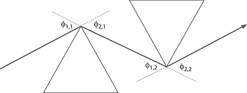
FIGURE 4.10 Double-prism pulse compressor.

Images

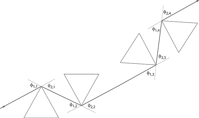
FIGURE 4.11 Four-prism pulse compressor obtained by symmetrically unfolding the double-prism configuration.

it is immediately apparent that the generation of ultrashort time pulses (Δt) requires the simultaneous generation of a very wide spectral distribution (Δν). From the cavity linewidth equation

Δ λ = Δ θ (\nabla λ θ) - 1

$Δ λ = Δ θ (\nabla_{λ} θ)^{- 1}$

that can be expressed in the frequency domain as

Δ v = (c λ 2) Δ θ (\nabla λ θ) - 1 (4.63)

$Δ v = (\frac{c}{λ^{2}}) Δ θ (\nabla_{λ} θ)^{- 1} (4.63)$

it is also clear that the generation of very wide spectral emission requires the least amount of intracavity dispersion.

Pulse compression in ultrashort pulse, or femtosecond, lasers requires the control of the first, second, and third derivatives of the intracavity dispersion (see, e.g., Diels and Rudolph 2006). Using the identity (Duarte 1987a)

\nabla n ϕ 2, m = \nabla λ ϕ 2, m (\nabla λ n m) - 1 (4.64)

$\nabla_{n^{}} ϕ_{2, m} = \nabla_{λ^{}} ϕ_{2, m} (\nabla_{λ} n_{m})^{- 1} (4.64)$

the generalized single-pass dispersion equation

\nabla λ ϕ 2, m = H 2, m \nabla λ n m + (k 1, m k 2, m) - 1 [H 1, m \nabla λ n m \pm \nabla λ ϕ 2, (m - 1)]

$\nabla_{λ^{}} ϕ_{2, m} = ℋ_{2, m} \nabla_{λ} n_{m} + (k_{1, m} k_{2, m})^{- 1} [ℋ_{1, m} \nabla_{λ} n_{m} \pm \nabla_{λ^{}} ϕ_{2, (m - 1)}]$

can be restated as (Duarte 2009)

\nabla n ϕ 2, m = H 2, m + (M) - 1 [H 1, m \pm \nabla n ϕ 2, (m - 1)] (4.65)

$\nabla_{n^{}} ϕ_{2, m} = H_{2, m} + (ℳ)^{- 1} [H_{1, m} \pm \nabla_{n^{}} ϕ_{2, (m - 1)}] (4.65)$

where:

(M) - 1 = k - 1 1 m k - 1 2 m (4.66)

$(ℳ)^{- 1} = k_{1 m}^{- 1} k_{2 m}^{- 1} (4.66)$

Thus, the second derivative of the refraction angle, corresponding to r = 2, or the first derivative of the dispersion ∇_nϕ_2,m, is given by (Duarte 1987a)

\nabla 2 n ϕ 2, m = \nabla n H 2, m + (\nabla n M - 1) [H 1, m \pm \nabla n ϕ 2, (m - 1)] + (M - 1) [\nabla n H 1, m \pm \nabla 2 n (ϕ 2, (m - 1)] (4.67)

$\begin{matrix} \nabla_{n^{}}^{2} ϕ_{2, m} & = & \nabla_{n} ℋ_{2, m} \\ + (\nabla_{n} ℳ^{- 1}) [H_{1, m} \pm \nabla_{n^{}} ϕ_{2, (m - 1)}] \\ + (ℳ^{- 1}) [\nabla_{n} ℋ_{1, m} \pm \nabla_{n^{(}}^{2} ϕ_{2, (m - 1)}] \end{matrix} (4.67)$

The second derivative of the dispersion ∇_nϕ_2,m, corresponding to r = 3, is given by (Duarte 2009)

\nabla 3 n (ϕ 2, m = \nabla 2 n H 2, m + (\nabla 2 n M - 1) [H 1, m \pm \nabla n ϕ 2, (m - 1)] + 2 (\nabla n M - 1) [\nabla n H 1, m \pm \nabla 2 n (ϕ 2, (m - 1)] + (M - 1) [\nabla 2 n H 1, m \pm \nabla 3 n (ϕ 2, (m - 1)] (4.68)

$\begin{matrix} \nabla_{n^{(}}^{3} ϕ_{2, m} & = & \nabla_{n}^{2} H_{2, m} \\ + (\nabla_{n}^{2} ℳ^{- 1}) [H_{1, m} \pm \nabla_{n^{}} ϕ_{2, (m - 1)}] \\ + 2 (\nabla_{n} ℳ^{- 1}) [\nabla_{n} H_{1, m} \pm \nabla_{n^{(}}^{2} ϕ_{2, (m - 1)}] \\ + (ℳ^{- 1}) [\nabla_{n}^{2} ℋ_{1, m} \pm \nabla_{n^{(}}^{3} ϕ_{2, (m - 1)}] \end{matrix} (4.68)$

The third derivative of the dispersion ∇_nϕ_2,m, corresponding to r = 4, is given by (Duarte 2009)

\nabla 4 n (ϕ 2, m = \nabla 3 n H 2, m + (\nabla 3 n M - 1) [H 1, m \pm \nabla n ϕ 2, (m - 1)] + 3 (\nabla 2 n M - 1) [\nabla n H 1, m \pm \nabla 2 n (ϕ 2, (m - 1)] + 3 (\nabla n M - 1) [\nabla 2 n H 1, m \pm \nabla 3 n (ϕ 2, (m - 1)] + (M - 1) [\nabla 3 n H 1, m \pm \nabla 4 (n ϕ 2, (m - 1)] (4.69)

$\begin{matrix} \nabla_{n^{(}}^{4} ϕ_{2, m} & = & \nabla_{n}^{3} H_{2, m} \\ + (\nabla_{n}^{3} ℳ^{- 1}) [H_{1, m} \pm \nabla_{n^{}} ϕ_{2, (m - 1)}] \\ + 3 (\nabla_{n}^{2} ℳ^{- 1}) [\nabla_{n} ℋ_{1, m} \pm \nabla_{n^{(}}^{2} ϕ_{2, (m - 1)}] \\ + 3 (\nabla_{n} ℳ^{- 1}) [\nabla_{n}^{2} ℋ_{1, m} \pm \nabla_{n^{(}}^{3} ϕ_{2, (m - 1)}] \\ + (ℳ^{- 1}) [\nabla_{n}^{3} H_{1, m} \pm \nabla_{n}^{4_{(}} ϕ_{2, (m - 1)}] \end{matrix} (4.69)$

The fourth derivative of the dispersion ∇_nϕ_2,m, corresponding to r = 5, is given by (Duarte 2009)

\nabla 5 n (ϕ 2, m = \nabla 4 n H 2, m + (\nabla 4 n M - 1) [H 1, m \pm \nabla n ϕ 2, (m - 1)] + 4 (\nabla 3 n M - 1) [\nabla n H 1, m \pm \nabla 2 n (ϕ 2, (m - 1)] + 6 (\nabla 2 n M - 1) [\nabla 2 n H 1, m \pm \nabla 3 n (ϕ 2, (m - 1)] + 4 (\nabla n M - 1) [\nabla 3 n H 1, m \pm \nabla 4 (n ϕ 2, (m - 1)] + (M - 1) [\nabla 4 n H 1, m \pm \nabla 5 n (ϕ 2, (m - 1)] (4.70)

$\begin{matrix} \nabla_{n^{(}}^{5} ϕ_{2, m} & = & \nabla_{n}^{4} ℋ_{2, m} + (\nabla_{n}^{4} ℳ^{- 1}) [ℋ_{1, m} \pm \nabla_{n^{}} ϕ_{2, (m - 1)}] \\ + 4 (\nabla_{n}^{3} ℳ^{- 1}) [\nabla_{n} H_{1, m} \pm \nabla_{n^{(}}^{2} ϕ_{2, (m - 1)}] \\ + 6 (\nabla_{n}^{2} ℳ^{- 1}) [\nabla_{n}^{2} H_{1, m} \pm \nabla_{n^{(}}^{3} ϕ_{2, (m - 1)}] \\ + 4 (\nabla_{n} ℳ^{- 1}) [\nabla_{n}^{3} ℋ_{1, m} \pm \nabla_{n}^{4_{(}} ϕ_{2, (m - 1)}] \\ + (ℳ^{- 1}) [\nabla_{n}^{4} ℋ_{1, m} \pm \nabla_{n^{(}}^{5} ϕ_{2, (m - 1)}] \end{matrix} (4.70)$

The fifth derivative of the dispersion ∇_λϕ_2,m, corresponding to r = 6, is given by

\nabla 6 n (ϕ 2, m = \nabla 5 n H 2, m + (\nabla 5 n M - 1) [H 1, m \pm \nabla n ϕ 2, (m - 1)] + 5 (\nabla 4 n M - 1) [\nabla n H 1, m \pm \nabla 2 n (ϕ 2, (m - 1)] + 10 (\nabla 3 n M - 1) [\nabla 2 n H 1, m \pm \nabla 3 n (ϕ 2, (m - 1)] + 10 (\nabla 2 n M - 1) [\nabla 3 n H 1, m \pm \nabla 4 n (ϕ 2, (m - 1)] + 5 (\nabla n M - 1) [\nabla 4 n H 1, m \pm \nabla 5 n (ϕ 2, (m - 1)] + (M - 1) [\nabla 5 n H 1, m \pm \nabla 6 n (ϕ 2, (m - 1)] (4.71)

$\begin{matrix} \nabla_{n^{(}}^{6} ϕ_{2, m} & = & \nabla_{n}^{5} ℋ_{2, m} + (\nabla_{n}^{5} ℳ^{- 1}) [ℋ_{1, m} \pm \nabla_{n^{}} ϕ_{2, (m - 1)}] \\ + 5 (\nabla_{n}^{4} ℳ^{- 1}) [\nabla_{n} ℋ_{1, m} \pm \nabla_{n^{(}}^{2} ϕ_{2, (m - 1)}] \\ + 10 (\nabla_{n}^{3} ℳ^{- 1}) [\nabla_{n}^{2} H_{1, m} \pm \nabla_{n^{(}}^{3} ϕ_{2, (m - 1)}] \\ + 10 (\nabla_{n}^{2} ℳ^{- 1}) [\nabla_{n}^{3} H_{1, m} \pm \nabla_{n^{(}}^{4} ϕ_{2, (m - 1)}] \\ + 5 (\nabla_{n} ℳ^{- 1}) [\nabla_{n}^{4} ℋ_{1, m} \pm \nabla_{n^{(}}^{5} ϕ_{2, (m - 1)}] \\ + (ℳ^{- 1}) [\nabla_{n}^{5} ℋ_{1, m} \pm \nabla_{n^{(}}^{6} ϕ_{2, (m - 1)}] \end{matrix} (4.71)$

The sixth derivative of the dispersion ∇_nϕ_2,m, corresponding to r = 7, is given by (Duarte 2013)

\nabla 7 n ϕ 2, m = \nabla 6 n H 2, m + (\nabla 6 n M - 1) [H 1, m \pm \nabla n ϕ 2, (m - 1)] + 6 (\nabla 5 n M - 1) [\nabla n H 1, m \pm \nabla 2 n ϕ 2, (m - 1)] + 15 (\nabla 4 n M - 1) [\nabla 2 n H 1, m \pm \nabla 3 n ϕ 2, (m - 1)] + 20 (\nabla 3 n 9 4 - 1) [\nabla 3 n H 1, m \pm \nabla 4 (n ϕ 2, (m - 1)] + 15 (\nabla 2 n M - 1) [\nabla 4 n H 1, m \pm \nabla 5 n ϕ 2, (m - 1)] + 6 (\nabla n M - 1) [\nabla 5 n H 1, m \pm \nabla 6 n ϕ 2, (m - 1)] + (M - 1) [\nabla 6 n H 1, m \pm \nabla 7 n ϕ 2, (m - 1)] (4.72)

$\begin{matrix} \nabla_{n^{}}^{7} ϕ_{2, m} & = & \nabla_{n}^{6} H_{2, m} + (\nabla_{n}^{6} ℳ^{- 1}) [H_{1, m} \pm \nabla_{n^{}} ϕ_{2, (m - 1)}] \\ + 6 (\nabla_{n}^{5} ℳ^{- 1}) [\nabla_{n} H_{1, m} \pm \nabla_{n^{}}^{2} ϕ_{2, (m - 1)}] \\ + 15 (\nabla_{n}^{4} ℳ^{- 1}) [\nabla_{n}^{2} ℋ_{1, m} \pm \nabla_{n^{}}^{3} ϕ_{2, (m - 1)}] \\ + 20 (\nabla_{n}^{3} 9 4^{- 1}) [\nabla_{n}^{3} ℋ_{1, m} \pm \nabla_{n}^{4_{(}} ϕ_{2, (m - 1)}] \\ + 15 (\nabla_{n}^{2} ℳ^{- 1}) [\nabla_{n}^{4} H_{1, m} \pm \nabla_{n^{}}^{5} ϕ_{2, (m - 1)}] \\ + 6 (\nabla_{n} ℳ^{- 1}) [\nabla_{n}^{5} H_{1, m} \pm \nabla_{n^{}}^{6} ϕ_{2, (m - 1)}] \\ + (ℳ^{- 1}) [\nabla_{n}^{6} ℋ_{1, m} \pm \nabla_{n^{}}^{7} ϕ_{2, (m - 1)}] \end{matrix} (4.72)$

Hence, it can be seen that from the second term on, the numerical factors can be predetermined from Pascal’s triangle relative to N, where (N + 1) is the order of the derivative (Duarte 2009). Observing the progression of the higher derivatives, a generalized expression is found to be (Duarte 2013)

\nabla' n ϕ 2, m = \nabla r - 1 n H 2, m + (M) - 1 (\nabla n + ζ) r - 1 (4.73)

$\nabla_{n^{}}^{'} ϕ_{2, m} = \nabla_{n}^{r - 1} H_{2, m} + (M)^{- 1} (\nabla_{n} + ζ)^{r - 1} (4.73)$

where

ζ S = \nabla s n H 1, m \pm \nabla s + 1 n ϕ 2, (m - 1) (4.74)

$ζ^{S} = \nabla_{n}^{s} H_{1, m} \pm \nabla_{n}^{s + 1} ϕ_{2, (m - 1)} (4.74)$

ζ 0 = 1 = H 1, m \pm \nabla n ϕ 2, (m - 1) (4.75)

$ζ^{0} = 1 = ℋ_{1, m} \pm \nabla_{n^{}} ϕ_{2, (m - 1)} (4.75)$

Here, when writing the expansion in r, in Equation 4.73, the term ζ⁰ = 1 must be included as defined in Equation 4.75. Also, in Equation 4.74, the maximum value of the exponent is s = (r − 1).

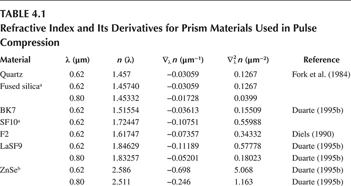
These equations represent the complete description of the generalized multiple-prism dispersion theory applicable to pulse compression prismatic arrays in femto-second, or ultrashort, pulse lasers and nonlinear optics. Exact numerical calculations to determine ∇_nϕ_2,3 and ∇2ntϕ2,m $\nabla_{n}^{2} t ϕ_{2, m}$ , for m = 1, 2, 3, 4, were performed by Duarte (1990b). In these calculations, the angle of incidence was deviated by minute amounts from the Brewster angle of incidence. Duarte (2009) provides the exact values, as a function of the refractive index n, for ∇_λϕ_2,m, ∇2ntϕ2,m $\nabla_{n}^{2} t ϕ_{2, m}$ and ∇3ntϕ2,m $\nabla_{n}^{3} t ϕ_{2, m}$ . Simplifying assumptions include incidence at the Brewster angle of incidence, prisms of identical isosceles geometry, and made of the same material with refractive index n_m = n.

Furthermore, these equations have been applied to yield specific numerical results (Duarte 1987a, 1990b): for example, Osvay et al. (2004, 2005) have used the lower order derivatives, given here, in practical femtosecond lasers to determine dispersions and laser pulse durations for double-prism compressors with excellent agreement between theory and experiments. Table 4.1 provides the refractive index and dispersions for some prism materials used in prismatic pulse compressors.

4.5.1 Example

A four-prism compressor (Fork et al. 1984) is formed by unfolding the double-prism configuration about a symmetry axis perpendicular to the exit beam depicted in Figure 4.10, as illustrated in Figure 4.11. For exactly balanced compensating prism arrays composed of two pairs of compensating prisms, it can be shown that (Duarte 1987a, 2009)

\nabla n ϕ 2, 1 = \nabla n ϕ 2, 3 = 2 (4.76)

$\nabla_{n^{}} ϕ_{2, 1} = \nabla_{n^{}} ϕ_{2, 3} = 2 (4.76)$

\nabla 2 n ϕ 2, 1 = \nabla 2 n ϕ 2, 3 = (4 n - 2 n - 3) (4.77)

$\nabla_{n^{}}^{2} ϕ_{2, 1} = \nabla_{n^{}}^{2} ϕ_{2, 3} = (4 n - 2 n^{- 3}) (4.77)$

\nabla 3 n ϕ 2, 1 = \nabla 3 n ϕ 2, 3 = (24 n 2 + 8 n 0 - 12 n - 2 + 6 n - 4 + 6 n - 6) (4.78)

$\nabla_{n^{}}^{3} ϕ_{2, 1} = \nabla_{n^{}}^{3} ϕ_{2, 3} = (24 n^{2} + 8 n^{0} - 12 n^{- 2} + 6 n^{- 4} + 6 n^{- 6}) (4.78)$

TABLE 4.1
Refractive Index and Its Derivatives for Prism Materials Used in Pulse Compression

Images

\nabla n ϕ 2, 2 = \nabla n ϕ 2, 4 = 0 (4.79)

$\nabla_{n^{}} ϕ_{2, 2} = \nabla_{n^{}} ϕ_{2, 4} = 0 (4.79)$

\nabla 2 n ϕ 2, 2 = \nabla 2 n ϕ 2, 4 = 0 (4.80)

$\nabla_{n^{}}^{2} ϕ_{2, 2} = \nabla_{n^{}}^{2} ϕ_{2, 4} = 0 (4.80)$

\nabla 3 n ϕ 2, 2 = \nabla 3 n ϕ 2, 4 = 0 (4.81)

$\nabla_{n^{}}^{3} ϕ_{2, 2} = \nabla_{n^{}}^{3} ϕ_{2, 4} = 0 (4.81)$

A six-prism pulse compressor has been used in semiconductor laser pulse compression by Pang et al. (1992). Certainly, the equations provided here can be applied to prismatic pulse compressors comprising any number of prisms and deployed in any suitable geometry.

4.6 Applications of Multiple-Prism Arrays

So far, the use of multiple-prism arrays as intracavity beam expanders in narrow-linewidth tunable laser oscillators and as pulse compressors in ultrafast lasers has been examined. However, as discussed by Duarte (2000), multiple-prism arrays as one-dimensional telescopes, or beam expanders, have found a plethora of alternative applications:

Extracavity double-prism beam expander to correct the ellipticity of laser beams generated by semiconductor lasers (Maker and Ferguson 1989). These expanders make use of the prism pairs first introduced by Brewster (1813).
Generalized laser beam shaping devices as discussed by Duarte (1987b, 1995c).
Beam expanding devices for optical computing (Lohmann and Stork 1989).
One-dimensional beam expanders yielding extremely elongated Gaussian beams, with height-to-width ratios in the 1:1000 to 1:3000 range for microscopy applications (Duarte 1987a, 1993, 1995b). This includes characterization of transmission and reflection imaging surfaces (see Chapter 10). Note that this type of illumination is also known in the literature as light sheet illumination and selective plane illumination.
Multiple-prism beam expansion for N-slit interferometry (Duarte 1991, 1993).
One-dimensional multiple-prism telescopes in conjunction with digital detectors (Duarte 1993, 1995b). This includes applications in conjunction with transmission grating in areas of wavelength measurements (Duarte 1995b) and secure optical communications (Duarte 2002; Duarte et al. 2010, 2011).
One-dimensional beam expansion for application in laser printers for imaging applications, also known as laser sensitometers (Duarte 2001a; Duarte et al. 2005).
Beam expansion for imaging systems used in astronomy, particularly in the subfield of astrometry (Sirat et al. 2005).
Multiple-prism assemblies for Amici prisms for dispersion correction in direct vision instrumentation for astronomy applications (Wynne 1997).

Problems

4.1 Show that Equation 4.11 can also be expressed in its explicit form of Equation 4.14.

4.2 Show that for orthogonal beam exit Equation 4.14 reduces to Equation 4.17.

4.3 Show that for prism with (α₁ = α₂ = α₃ = ... = α_m and deployed for Brewster’s angle of incidence, Equation 4.17 can be restated as Equation 4.19.

4.4 Design a three-prism beam expander with ∇_λΦ_P = 0 for M ≈ 70. Assume λ = 590 nm, n = 1.5167 and w = 100 μm.

4.5 Show that for m = 1, orthogonal beam exit, and Brewster’s angle of incidence, Equation 4.17 reduces to Equation 4.38.

4.6 Expand Equation 4.73 for r = 7 to arrive at Equation 4.72.

..................Content has been hidden....................

You can't read the all page of ebook, please click here login for view all page.

Table of Contents for
Chapter 4 The Physics of Multiple- Prism Optics

4

The Physics of Multiple- Prism Optics

4.1 Introduction

4.2 Generalized Multiple-Prism Dispersion

4.2.1 Double-Pass Generalized Multiple-Prism Dispersion

4.2.2 Multiple Return-Pass Generalized Multiple-Prism Dispersion

4.2.3 Single-Prism Equations

4.3 Multiple-Prism Dispersion Linewidth Narrowing

4.3.1 Mechanics of Linewidth Narrowing in Optically Pumped Pulsed Laser Oscillators

4.3.2 Design of Zero-Dispersion Multiple-Prism Beam Expanders

4.3.2.1 Example

4.3.2.2 Example

4.4 Dispersion of Amici, or Compound, Prisms

4.4.1 Example

4.5 Multiple-Prism Dispersion and Pulse Compression

4.5.1 Example

4.6 Applications of Multiple-Prism Arrays

Problems

Table of Contents for Chapter 4 The Physics of Multiple- Prism Optics

Create new playlist

Sign In

Sign Up

Table of Contents for
Chapter 4 The Physics of Multiple- Prism Optics