Chapter 3 The Uncertainty Principle in Optics

Search in book...
Toggle Font Controls
Create new playlist

Name your new playlist

Playlist description (optional)
Sign In

Email address

Password

Forgot Password?

or

Continue with Facebook

Continue with Google
Sign Up

Full Name

Email address

Confirm Email Address

Password

or

Continue with Facebook

Continue with Google

Heisenberg’s uncertainty principle (Heisenberg 1927) is of fundamental importance to optics and to laser optics in particular. Here, optical arguments are applied to outline an approximate derivation of the uncertainty principle.

3.1.1 The Wave Character of Particles

The quantum energy of a particle is given by the well-known quantum energy equation

E = h v (3.1)

$E = h v (3.1)$

where:

h is Planck’s constant

Equating this to the relativistic energy E = mc² and using the identity λ = c/ν, an expression for the momentum of a particle can be given as

p = \frac{h}{λ} (3.2)

$p = \frac{h}{λ} (3.2)$

which, using the identity

k = \frac{2 π}{λ} (3.3)

$k = \frac{2 π}{λ} (3.3)$

can be restated as

p = ħ k (3.4)

$p = ħ k (3.4)$

This momentum equation was applied to particles, such as electrons, by de Broglie (Haken 1981). Thus, wave properties such as frequency and wavelength were attributed to the motion of particles.

3.1.2 The Diffraction Identity and the Uncertainty Principle

In his discussion of position and momentum, Feynman considers the relative uncertainty in the wavelength that can be measured with a given grating (Feynman et al., 1965). Using such approach, he arrives at an expression for the resolving power of a diffraction grating: Δλ/λ. His discussion is then extended to include the length of a wave train in order to derive an identity for Δλ/λ². Here, the origin of this expression is examined from an interferometric perspective.

The generalized one-dimensional interferometric equation derived using Dirac’s notation is given by (Duarte 1991)

| 〈 x | s 〉 |^{2} = \sum_{j = 1}^{N} Ψ (r_{j})^{2} + 2 \sum_{j = 1}^{N} Ψ (r_{j}) [\sum_{m = j + 1}^{N} Ψ (r_{m}) \cos (Ω_{m} - Ω_{j})] (3.5)

$| 〈 x | s 〉 |^{2} = \sum_{j = 1}^{N} Ψ (r_{j})^{2} + 2 \sum_{j = 1}^{N} Ψ (r_{j}) [\sum_{m = j + 1}^{N} Ψ (r_{m}) \cos (Ω_{m} - Ω_{j})] (3.5)$

The interference term in this equation can be expressed as (Duarte 1997)

\cos [(θ_{m} - θ_{j}) \pm (ϕ_{m} - ϕ_{j})] = \cos (| l_{m} - l_{m - 1} | k_{1} \pm | L_{m} - L_{m - 1} | k_{2}) (3.6)

$\cos [(θ_{m} - θ_{j}) \pm (ϕ_{m} - ϕ_{j})] = \cos (| l_{m} - l_{m - 1} | k_{1} \pm | L_{m} - L_{m - 1} | k_{2}) (3.6)$

where:

k_{1} = \frac{2 π n_{1}}{λ_{v}}

$k_{1} = \frac{2 π n_{1}}{λ_{v}}$

and

k_{2} = \frac{2 π n_{2}}{λ_{v}}

$k_{2} = \frac{2 π n_{2}}{λ_{v}}$

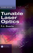
are the wave numbers for the two optical regions, defined in Figure 3.1 (see Chapter 2 for further details). Also, |l_m - l_m_-1| and |L_m - L_m_-1| are the corresponding path differences. Since it can be shown that maxima can occur at

(| l_{m} - l_{m - 1} | n_{1} \pm | L_{m} - L_{m - 1} | n_{2}) \frac{2 π}{λ_{v}} = M π (3.7)

$(| l_{m} - l_{m - 1} | n_{1} \pm | L_{m} - L_{m - 1} | n_{2}) \frac{2 π}{λ_{v}} = M π (3.7)$

where:

M = 0, ±2, ±4, ±6, …

it can be shown that

d_{m} (n_{1} \sin Θ_{m} \pm n_{2} \sin Φ_{m}) \frac{2 π}{λ_{v}} = M π (3.8)

$d_{m} (n_{1} \sin Θ_{m} \pm n_{2} \sin Φ_{m}) \frac{2 π}{λ_{v}} = M π (3.8)$

which, for n₁ = n₂ = 1 and λ = λ_v, reduces to

d_{m} (\sin Θ_{m} \pm \sin Φ_{m}) k = M π (3.9)

$d_{m} (\sin Θ_{m} \pm \sin Φ_{m}) k = M π (3.9)$

that can be expressed as the well-known grating equation

d_{m} (\sin Θ_{m} \pm \sin Φ_{m}) = m λ (3.10)

$d_{m} (\sin Θ_{m} \pm \sin Φ_{m}) = m λ (3.10)$

where:

m = 0, ±1, ±2, ±3, ...

Images

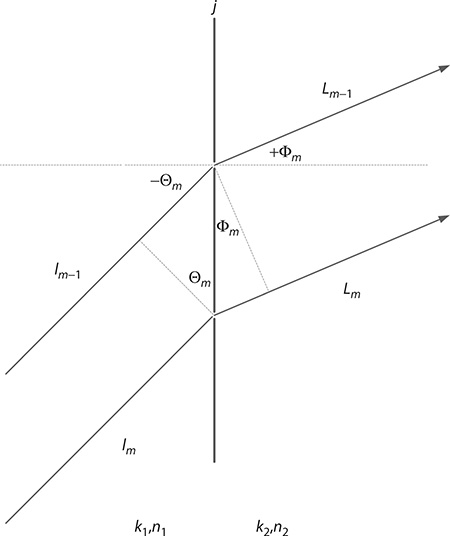
FIGURE 3.1 Boundary at a transmission grating depicting corresponding path differences. Further details on the geometry of the transmission grating are given in Chapter 2.

For a grating deployed in the reflection domain, and at Littrow configuration, Θ_m = Φ_m = Θ so that the grating equation reduces to

2 d \sin Θ = m λ (3.11)

$2 d \sin Θ = m λ (3.11)$

Using this equation, one can consider an expanded light beam incident on a reflection grating as illustrated in Figure 3.2. For an infinitesimal change in wavelength

λ_{1} = \frac{2 d}{m} (\frac{Δ x_{1}}{l}) (3.12)

$λ_{1} = \frac{2 d}{m} (\frac{Δ x_{1}}{l}) (3.12)$

λ_{2} = \frac{2 d}{m} (\frac{Δ x_{2}}{l}) (3.13)

$λ_{2} = \frac{2 d}{m} (\frac{Δ x_{2}}{l}) (3.13)$

where:

l is the grating length

Δx is the path difference

From the geometry of Figure 3.2 and the corresponding grating equation for the Littrow configuration (Equation 3.11),

\frac{2 d}{m} = \frac{l λ}{Δ x} (3.14)

$\frac{2 d}{m} = \frac{l λ}{Δ x} (3.14)$

Images

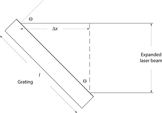
FIGURE 3.2 Path differences in a diffraction grating of the reflective class in Littrow configuration. From the geometry, sin Θ = (Δx/l).

Then, it follows that

Δ λ = \frac{l λ}{Δ x} (\frac{Δ x_{1} - Δ x_{2}}{l}) (3.15)

$Δ λ = \frac{l λ}{Δ x} (\frac{Δ x_{1} - Δ x_{2}}{l}) (3.15)$

In order to distinguish between a maximum and a minimum, the difference in path differences should be equal to a single wavelength, that is,

(Δ x_{1} - Δ x_{2}) \approx λ (3.16)

$(Δ x_{1} - Δ x_{2}) \approx λ (3.16)$

Hence, Equation 3.15 reduces to the well-known diffraction identity

Δ λ \approx \frac{λ^{2}}{Δ x} (3.17)

$Δ λ \approx \frac{λ^{2}}{Δ x} (3.17)$

which in turn leads to

Δ v \approx \frac{c}{Δ x} (3.18)

$Δ v \approx \frac{c}{Δ x} (3.18)$

Assuming a grating composed of uniform and equally spaced slits of width d, separated themselves by a distance d, the total length of the grating can be stated as l ≈ 2Nd, where N is the total number of slits. Hence, the path difference can be written as Δx ≈ mNλ so that Equation 3.17 can also be expressed as

\frac{Δ λ}{λ^{2}} \approx \frac{1}{m N λ} (3.19)

$\frac{Δ λ}{λ^{2}} \approx \frac{1}{m N λ} (3.19)$

and multiplication by λ yields

\frac{Δ λ}{λ} \approx \frac{1}{m N} (3.20)

$\frac{Δ λ}{λ} \approx \frac{1}{m N} (3.20)$

which is known as the resolving power of a diffraction grating. Now, considering p = ħk for two slightly different wavelengths leads to

p_{1} - p_{2} = \frac{h (λ_{1} - λ_{2})}{λ_{1} λ_{2}} (3.21)

$p_{1} - p_{2} = \frac{h (λ_{1} - λ_{2})}{λ_{1} λ_{2}} (3.21)$

and since the difference between λ₁ and λ₂ is infinitesimal, this equation can be restated as

Δ p \approx h \frac{Δ λ}{λ^{2}} (3.22)

$Δ p \approx h \frac{Δ λ}{λ^{2}} (3.22)$

Substitution of Equation 3.22 into 3.17 leads to

Δ p Δ x \approx h (3.23)

$Δ p Δ x \approx h (3.23)$

which is known as Heisenberg’s uncertainty principle (Dirac 1978). This approach offers a geometrical perspective on the foundations of the uncertainty principle. It should also be noted that many authors also express the uncertainty principle in its minimum form where the right-hand side is given by ħ/2 rather than h:

Δ p Δ x \approx \frac{h}{2} (3.24)

$Δ p Δ x \approx \frac{h}{2} (3.24)$

This minimal version of the uncertainty principle, in addition to a generalized version, is discussed in Duarte (2014).

3.1.3 Alternative Versions of the Uncertainty Principle

In addition to Δp Δx ≈ h, the uncertainty principle can be expressed in various useful versions. Assuming an independent derivation, and using p = ħk, it can be expressed in its wavelength-spatial form:

Δ λ Δ x \approx λ^{2} (3.25)

$Δ λ Δ x \approx λ^{2} (3.25)$

which can also be stated in its frequency-spatial version:

Δ v Δ x \approx c (3.26)

$Δ v Δ x \approx c (3.26)$

which are Equations 3.17 and 3.18 in an alternative format. Using E = mc², the uncertainty principle can also be written in its energy–time form:

Δ E Δ t \approx h (3.27)

$Δ E Δ t \approx h (3.27)$

which, using the quantum energy E = hν, can be transformed to its frequency–time version:

Δ v Δ t \approx 1 (3.28)

$Δ v Δ t \approx 1 (3.28)$

This result is very important in the area of pulsed lasers and implies that a laser emitting a pulse of a given duration Δt has a minimum spectral linewidth Δν. It also implies that by measuring the width of the spectral emission the duration of that pulse can be determined. The time

Δ t \approx \frac{1}{Δ v} (3.29)

$Δ t \approx \frac{1}{Δ v} (3.29)$

is also known as the coherence time. From this time, the coherence length can be defined as

Δ x \approx \frac{c}{Δ v} (3.30)

$Δ x \approx \frac{c}{Δ v} (3.30)$

which is an alternative form of Equation 3.26. This equation has gigantic physical implications as it illustrates the fact that a single photon, with an infinitesimal narrow linewidth Δν, can have an enormous coherence length.

3.2 Applications of the Uncertainty Principle in Optics

In this section, some useful applications of the uncertainty principle in beam propagation and intracavity optics are considered.

3.2.1 Beam Divergence

If the uncertainty principle is assumed to be derived from independent and rigorous methods, then it can be used to derive some useful identities in optics. For example, starting from

Δ p Δ x \approx h

$Δ p Δ x \approx h$

the application of p = ħk yields

Δ k Δ x \approx 2 π (3.31)

$Δ k Δ x \approx 2 π (3.31)$

which leads directly to

Δ λ \approx \frac{λ^{2}}{Δ x}

$Δ λ \approx \frac{λ^{2}}{Δ x}$

For a diffraction-limited beam traveling in the z-direction

k_{x} = k \sin θ (3.32)

$k_{x} = k \sin θ (3.32)$

and/or a very small angle θ, we can write

k_{x} \approx k θ (3.33)

$k_{x} \approx k θ (3.33)$

Using Δk_xΔx ≈ 2π, it is readily seen that the beam has an angular divergence given by

Δ θ \approx \frac{λ}{Δ x} (3.34)

$Δ θ \approx \frac{λ}{Δ x} (3.34)$

This equation indicates that the angular spread of a propagating beam of wavelength λ is inversely proportional to its original width, that is, narrower beams exhibit a larger angular spread or divergence (see Figure 3.3). Also it states that the light of shorter wavelength experiences less beam divergence, which is a well-known experimental fact in laser physics (see Figure 3.4).

Images

FIGURE 3.3 Beam divergence for two different apertures at wavelength λ. (a) An expanded laser beam is incident on a microhole of diameter 2w. (b) The same laser beam is incident on a microhole of diameter 4w.

Images

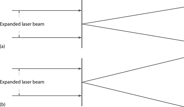
FIGURE 3.4 Beam divergence for (a) λ = 450 nm and (b) λ = 650 nm. In both cases, an expanded laser beam is incident on identical microholes of diameter 2w.

Equation 3.34 has the same form of the classical equation for beam divergence (Duarte 1990):

Δ θ = \frac{λ}{π w} [1 + (\frac{L_{ℛ} R}{B})^{2} + (\frac{A L_{ℛ} R}{B})^{2}]^{1 / 2} (3.35)

$Δ θ = \frac{λ}{π w} [1 + (\frac{L_{ℛ} R}{B})^{2} + (\frac{A L_{ℛ} R}{B})^{2}]^{1 / 2} (3.35)$

where:

w is the beam waist

L_ℛ = (πw²/λ) is the Rayleigh length

A and B are spatial propagation parameters defined in Chapter 6

For well-chosen experimental conditions, the second and third terms in the parentheses of Equation 3.35 approach zero so that

Δ θ \approx \frac{λ}{π w} (3.36)

$Δ θ \approx \frac{λ}{π w} (3.36)$

and the beam divergence is said to approach its diffraction limit. The equivalence of Equations 3.34 and 3.36 is self evident.

The generalized interference equation

| 〈 x | s 〉 |^{2} = \sum_{j = 1}^{N} Ψ (r_{j})^{2} + 2 \sum_{j = 1}^{N} Ψ (r_{j}) [\sum_{m = j + 1}^{N} Ψ (r_{m}) \cos (Ω_{m} - Ω_{j})]

$| 〈 x | s 〉 |^{2} = \sum_{j = 1}^{N} Ψ (r_{j})^{2} + 2 \sum_{j = 1}^{N} Ψ (r_{j}) [\sum_{m = j + 1}^{N} Ψ (r_{m}) \cos (Ω_{m} - Ω_{j})]$

was previously used to derive Δλ ≈ λ²/Δx, which eventually leads to ΔpΔx ≈ h and subsequently leads to an expression to the diffraction limited beam divergence.

3.2.1.1 Example

Here, we estimate the divergence of a coherent beam as it propagates in space using the one-dimensional generalized interferometric equation. For instance, at λ = 632.82 nm, a beam with an original dimension of 2w₀ = 200 μm can be estimated via Equation 3.5 to spread to 2w ≈ 1.89 mm (full width at half maximum [FWHM]) following a propagation of 0.5 m using an approximate graphical method (see Figure 3.5). The same beam can be estimated to increase further to 2w ≈ 18.9 mm (FWHM) following a propagation of 5 m. Using the dimensions of the beam waist w, and simple geometry, this yields an approximate beam divergence of Δθ ≈ 1.9 mrad. Alternatively, using Equation 3.36, the diffraction-limited beam divergence can be determined directly (for w₀ 100 nm and λ = 632.82 nm) as Δθ ≈ 2.01 mrad.

3.2.2 Beam Divergence and Astronomy

One application of the beam divergence equation relates to the angular resolution limit of telescopes used in astronomical observations. Reflection telescopes such as the Newtonian and Cassegrain telescopes are depicted in Figure 3.6 and discussed further in Chapter 6. The angular resolution that can be accomplished with these

Images

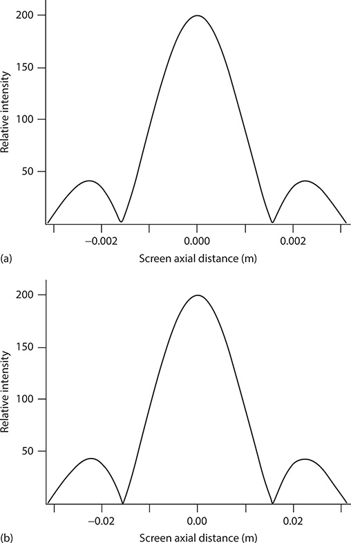
FIGURE 3.5 Beam divergence determined from the generalized interference equation. (a) Beam profile following propagation through a distance of 0.5 m. (b) Beam profile following propagation through a distance of 5 m. Here, w₀ = 100 μm and λ = 632.82 nm. Using the difference in beam waist w over the propagation distance, the beam divergence is determined to be Δθ ≈ 1.9 mrad.

telescopes under ideal conditions is approximately described by the diffraction limit given in Equation 3.36. That is, the smallest angular discrimination, or resolution limit, of a telescope with a diameter D = 2w is given by

Δ θ \approx \frac{2 λ}{π D} (3.37)

$Δ θ \approx \frac{2 λ}{π D} (3.37)$

Images

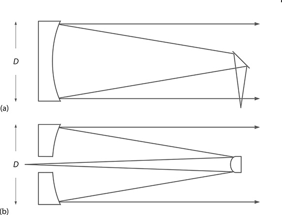
FIGURE 3.6 Reflection telescopes used in astronomical observations: (a) Newtonian telescope; (b) Cassegranian telescope.

This equation indicates that the two avenues to increase the angular resolution of a telescope are either to observe at shorter wavelengths or to increase the diameter of the telescope. The latter option has been adopted by optical designers that have built very large telescopes. At λ = 500 nm, the angular resolution for a telescope, with D = 10 m, is Δθ ≈ 3.18 × 10^-8 rad. For a diameter of D = 100 m, the angular resolution at the same wavelength becomes Δθ ≈ 3.18 × 10^-9 rad. Furthermore, for an hypothetical diameter of D = (1000/π) m, the angular resolution at λ = 500 nm becomes Δθ ≈ 1.00 × 10^-9 rad. In addition to better angular resolutions, large aperture telescopes provide increased signal since the area of collection increases substantially. In future, these ultralarge telescopes might become important in the search of exoplanets and in the study of fundamental physics phenomena during the very early stages of the universe.

Albeit great progress has been made in the construction of very large segmented mirrors, it might be a long time before telescopes of the extraordinary diameters mentioned here are built. In the meantime, interferometric telescopic arrays (see Chapter 11) can be used to significantly increase the light collection area and resolving power of individual telescopes. Such an array is the Very Large Telescope located at the Atacama Desert in northern Chile, which is composed of four telescopes, each telescope with a diameter of 8.2 m. As mentioned in Chapter 11, the first interferometric telescope was the Hanbury Brown–Twiss interferometer that, as emphasized by Feynman, is indeed a quantum optics instrument. We should also keep in mind that, as explicitly explained in this chapter, the angular resolution of telescopes can be explained either via quantum interferometric principles or via the uncertainty principle itself. Thus, it should not be surprising to see other quantum concepts adopted in the improvement of telescopic resolution.

3.2.2.1 Laser Guide Star

An important feature of large and very large terrestrial telescopes is the use of laser guide star techniques, in conjunction with adaptive optics, to correct for atmospheric turbulence. Atmospheric turbulence can seriously affect the optical homogeneity of the transmission medium as described and discussed in Chapter 10 from an interferometric perspective.

In guide star applications, the laser is tuned to the well-known atomic sodium 3²S_1/2 - 3²P_3/2 transition at λ = 588.9963 nm (also known as the sodium _D2 line; Mitchel and Zemansky 1971) and its beam is projected 90–100 km above the planetary surface. Emission from the sodium guide star induced by the illumination from the laser is collected by a Cassegrain telescope and used to characterize the atmospheric-induced distortions resulting from turbulence. The spatial information thus collected is used to drive the adaptive optics and compensate for atmospheric turbulence. In this application, three most important parameters of the laser are optical power, laser linewidth (Δν), and beam divergence (Δθ). More specifically, the laser should yield a diffraction-limited beam and single-longitudinal-mode emission (see Chapter 7).

Laser development for guide star applications originated with work on high-power tunable dye lasers (Everett 1989; Primmerman et al. 1991) and includes both pulsed and continuous-wave (CW) tunable lasers (Bass et al. 1992; Pique and Farinotti 2003). Alternatives to direct emission tunable organic dye lasers are frequency-doubled diode-pumped fiber Raman lasers (Feng et al. 2009; Henry et al. 2013).

The use of Amici prisms, or compounds prisms, for atmospheric dispersion corrections in astronomical applications is discussed in Chapter 4.

3.2.2.2 Example

Consider the propagation of a diffraction-limited laser beam over a distance of 95 km at λ = 589 nm for guide star applications in astronomy. A multiple-prism grating tunable laser oscillator (Duarte and Piper 1984; Duarte 1999) can be designed to provide single-longitudinal-mode oscillation at λ ≈ 589 nm in a laser with a beam divergence, which is nearly diffraction limited. Thus, its divergence is characterized by Δθ ≈ (λ/πw). For a beam waist w ≈ 125 μm, the corresponding beam divergence becomes Δθ ≈ 1.5 mrad. If the beam of this oscillator were to be propagated over a distance of 95 km, it would illuminate a circle of nearly 285 m in diameter. This would yield a very weak power density. If, however, the beam is expanded without introducing further divergence by a factor of M ≈ 200, then the new beam divergence becomes Δθ ≈ (λ/Mπw). Now, as a consequence of the beam expansion, the beam diameter at the required propagation distance becomes about 1.42 m, which is close to the dimensions needed to achieve the necessary power densities with existing high-power tunable lasers. It should be mentioned that the beam magnification factors of about 200 are not difficult to attain. Further, for this type of application, the narrow-linewidth oscillator emission is augmented at amplifier stages, where the beam also increases its dimensions, thus reducing the requirements on M.

3.3 The Interferometric Equation and the Uncertainty Principle

Previously, it has been shown that from the Dirac principle

〈 x | s 〉 = \sum_{j = 1}^{N} 〈 x | j 〉 〈 j | s 〉

$〈 x | s 〉 = \sum_{j = 1}^{N} 〈 x | j 〉 〈 j | s 〉$

the generalized interferometric equation

| 〈 x | s 〉 |^{2} = \sum_{j = 1}^{N} Ψ (r_{j})^{2} + 2 \sum_{j = 1}^{N} Ψ (r_{j}) [\sum_{m = j + 1}^{N} Ψ (r_{m}) \cos (Ω_{m} - Ω_{j})]

$| 〈 x | s 〉 |^{2} = \sum_{j = 1}^{N} Ψ (r_{j})^{2} + 2 \sum_{j = 1}^{N} Ψ (r_{j}) [\sum_{m = j + 1}^{N} Ψ (r_{m}) \cos (Ω_{m} - Ω_{j})]$

can be obtained (Duarte 1991, 1993). This equation, originally derived while considering single-photon propagation (Duarte 1991), has also been shown to accurately predict interferometric distributions generated by the interaction of ensembles of indistinguishable photons with N-slit arrays (Duarte 1993). Furthermore, as shown by Duarte (1992), and explained in Chapter 2, the phase term of this generalized interferometric equation can be used to derive the cavity linewidth equation:

Δ λ \approx Δ θ (\nabla_{λ} θ)^{- 1}

$Δ λ \approx Δ θ (\nabla_{λ} θ)^{- 1}$

where:

Δθ is the beam divergence

∇_λθ = (∂θ/∂θ), which is the intracavity angular dispersion

This equation has been used extensively to determine the emission linewidth in pulsed narrow-linewidth dispersive laser oscillators (Duarte 2003). As shown earlier in this chapter, the beam divergence term

Δ θ \approx \frac{λ}{π w}

$Δ θ \approx \frac{λ}{π w}$

can be distilled from the uncertainty principle

Δ p Δ x \approx h

$Δ p Δ x \approx h$

which itself can also be obtained in an approximate approach, starting from the phase term of the interferometric equation, thus emphasizing a fundamental connection between these two principles. Besides, as shown by example, an estimate of Δθ can be obtained directly from the interferometric distributions provided via the interferometric equation. The phase term of the interferometric equation is in itself created by the interaction of probability amplitudes via the mechanics of the basic Dirac quantum principle

〈 x | s 〉 = \sum_{j = 1}^{N} 〈 x | j 〉 〈 j | s 〉

$〈 x | s 〉 = \sum_{j = 1}^{N} 〈 x | j 〉 〈 j | s 〉$

where the probability amplitudes are represented by wave functions of ordinary wave optics (Dirac 1978):

〈 j | s 〉 = Ψ (r_{j, s}) e^{- i θ_{j}}

$〈 j | s 〉 = Ψ (r_{j, s}) e^{- i θ_{j}}$

〈 x | j 〉 = Ψ (r_{x, j}) e^{- i ϕ_{j}}

$〈 x | j 〉 = Ψ (r_{x, j}) e^{- i ϕ_{j}}$

This exposition indicates that interference, as described by the Dirac notation, has a central and crucial position at the foundations of quantum mechanics and its significance might even be deeper than the significance of the uncertainty principle itself. The importance of interference to quantum mechanical principles was first highlighted by Dirac (1978) and then by Feynman et al. (1965).

3.3.1 Quantum Cryptography

Quantum secure communications and quantum cryptography are subjects of intense research activity. In this regard, it should be mentioned that Heisenberg’s uncertainty principle is often associated with the essence of quantum cryptography (Bennett et al. 1992).

An alternative approach to describe the mechanics of quantum cryptography is to use the probability amplitude of entangled polarizations of quanta traveling in opposite directions (Ekert 1991). The probability amplitude for entangled polarizations of quanta traveling in opposite directions was first introduced in the form of (Ward 1949)

| s 〉 = (| x 〉_{1} | y 〉_{2} - | y 〉_{1} | x 〉_{2}) (3.38)

$| s 〉 = (| x 〉_{1} | y 〉_{2} - | y 〉_{1} | x 〉_{2}) (3.38)$

which following straightforward normalization becomes

| Ψ_{-} 〉 = \frac{1}{\sqrt{2}} (| x 〉_{1} | y 〉_{2} - | y 〉_{1} | x 〉_{2}) (3.39)

$| Ψ_{-} 〉 = \frac{1}{\sqrt{2}} (| x 〉_{1} | y 〉_{2} - | y 〉_{1} | x 〉_{2}) (3.39)$

which is the ubiquitous probability amplitude depicting quantum entanglement given in numerous research papers and textbooks (see, e.g., Mandel and Wolf 1995). This probability amplitude can be derived via Ward’s argument (Ward 1949), a Hamiltonian approach (Duarte 2014), or via a neat and transparent approach from an N-slit interferometric perspective (Duarte 2013, 2014) again utilizing the Dirac principle:

〈 x | s 〉 = \sum_{j = 1}^{N} 〈 x | j 〉 〈 j | s 〉

$〈 x | s 〉 = \sum_{j = 1}^{N} 〈 x | j 〉 〈 j | s 〉$

Briefly, the probability amplitude for a single photon to propagate from a source s to the interferometric plane configured by a detector d via apertures 1 and 2 is given by 〈d | s〉

〈 d | s 〉 = 〈 d | 2 〉 〈 2 | s 〉 + 〈 d | 1 〉 〈 1 | s 〉 (3.40)

$〈 d | s 〉 = 〈 d | 2 〉 〈 2 | s 〉 + 〈 d | 1 〉 〈 1 | s 〉 (3.40)$

Images

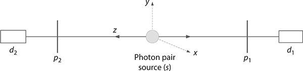
FIGURE 3.7 Generic experimental configuration of a source emitting two indistinguishable quanta traveling in opposite directions with entangled polarizations. This experimental arrangement is a simplified rendition of the original configuration introduced by Pryce and Ward.

For an experiment with a central photon source emitting indistinguishable quanta toward identical detectors (d₁ = d₂ d) positioned in opposite directions via polarization analyzers p₁ and p₂ (see Figure 3.7), the corresponding probability amplitude can be described as

〈 d | s 〉 = 〈 d | p_{2} 〉 〈 p_{2} | s 〉 + 〈 d | p_{1} 〉 〈 p_{1} | s 〉 (3.41)

$〈 d | s 〉 = 〈 d | p_{2} 〉 〈 p_{2} | s 〉 + 〈 d | p_{1} 〉 〈 p_{1} | s 〉 (3.41)$

In abstract form, this probability amplitude can be expressed as

| s 〉 = | p_{2} 〉 〈 p_{2} | s 〉 + | p_{1} 〉 〈 p_{1} | s 〉 (3.42)

$| s 〉 = | p_{2} 〉 〈 p_{2} | s 〉 + | p_{1} 〉 〈 p_{1} | s 〉 (3.42)$

Defining

| C_{1} 〉 = | p_{1} 〉 〈 p_{1} | s 〉 (3.43)

$| C_{1} 〉 = | p_{1} 〉 〈 p_{1} | s 〉 (3.43)$

and

| C_{2} 〉 = | p_{2} 〉 〈 p_{2} | s 〉 (3.44)

$| C_{2} 〉 = | p_{2} 〉 〈 p_{2} | s 〉 (3.44)$

Equation 3.42 can be expressed as

| s 〉 = | C_{2} 〉 + | C_{1} 〉 (3.45)

$| s 〉 = | C_{2} 〉 + | C_{1} 〉 (3.45)$

Using the Dirac identity applicable to the state of several similar particles

| X 〉 = | a_{1} 〉 | b_{2} 〉 | c_{3} 〉 ... | g_{n} 〉 (3.46)

$| X 〉 = | a_{1} 〉 | b_{2} 〉 | c_{3} 〉 ... | g_{n} 〉 (3.46)$

for quanta 1 and quanta 2, we can write

| C_{2} 〉 = | x 〉_{1} | y 〉_{2} (3.47)

$| C_{2} 〉 = | x 〉_{1} | y 〉_{2} (3.47)$

and

| C_{1} 〉 = | y 〉_{1} | x 〉_{2} (3.48)

$| C_{1} 〉 = | y 〉_{1} | x 〉_{2} (3.48)$

Substituting back in Equation 3.45, and following normalization, leads to

| Ψ_{+} 〉 = \frac{1}{\sqrt{2}} (| x 〉_{1} | y 〉_{2} + | y 〉_{1} | x 〉_{2}) (3.49)

$| Ψ_{+} 〉 = \frac{1}{\sqrt{2}} (| x 〉_{1} | y 〉_{2} + | y 〉_{1} | x 〉_{2}) (3.49)$

and its linear combination

| Ψ_{-} 〉 = \frac{1}{\sqrt{2}} (| x 〉_{1} | y 〉_{2} - | y 〉_{1} | x 〉_{2})

$| Ψ_{-} 〉 = \frac{1}{\sqrt{2}} (| x 〉_{1} | y 〉_{2} - | y 〉_{1} | x 〉_{2})$

An extension of the Ward probability amplitude is the probability amplitude for n entangled particles propagating in two different directions (Duarte 2013):

| Ψ 〉 = \frac{1}{\sqrt{2}} (| a 〉_{1} | b 〉_{2} | c 〉_{3} ... | g 〉_{n} \pm | a' 〉_{1} | b' 〉_{2} | c' 〉_{3} ... | g' 〉_{n}) (3.50)

$| Ψ 〉 = \frac{1}{\sqrt{2}} (| a 〉_{1} | b 〉_{2} | c 〉_{3} ... | g 〉_{n} \pm | a' 〉_{1} | b' 〉_{2} | c' 〉_{3} ... | g' 〉_{n}) (3.50)$

For N path alternatives, the overall probability amplitude is given by

| s 〉 = \sum_{j = 1}^{N} | C_{N + 1 - j} 〉 (3.51)

$| s 〉 = \sum_{j = 1}^{N} | C_{N + 1 - j} 〉 (3.51)$

where the first term of the path probability amplitude series can be written as

C_{N + 1 - j} = \prod_{m = 1}^{n} | γ 〉_{m} (3.52)

$C_{N + 1 - j} = \prod_{m = 1}^{n} | γ 〉_{m} (3.52)$

These are a series of probability amplitudes starting at C_N+1−j, with j = 1, and ending at C₁, which is reached when j = N. Here, n is the total number of quanta, which is an even number since quanta participate in pairs. For each pair (1, 2), (3, 4)...(n - 1, n), γ represents a pair of orthogonal polarization alternatives such as x and y, and ϕ and ϕ′.

For an even number of paths, the normalized probability amplitudes, designated by C_R, where R is a Roman numeral, have the form:

C_{R} = \frac{1}{\sqrt{N}} \sum_{m = 1}^{N} (\pm) C_{m} (3.53)

$C_{R} = \frac{1}{\sqrt{N}} \sum_{m = 1}^{N} (\pm) C_{m} (3.53)$

However, for N = 3,

C_{I} = \frac{1}{\sqrt{3}} (C_{3} + C_{2} + i C_{1}) (3.54)

$C_{I} = \frac{1}{\sqrt{3}} (C_{3} + C_{2} + i C_{1}) (3.54)$

C_{I I} = \frac{1}{\sqrt{3}} (C_{3} - C_{2} + i C_{1}) (3.55)

$C_{I I} = \frac{1}{\sqrt{3}} (C_{3} - C_{2} + i C_{1}) (3.55)$

C_{I I I} = \frac{1}{\sqrt{3}} (i C_{3} + j C_{2} + k C_{1}) (3.56)

$C_{I I I} = \frac{1}{\sqrt{3}} (i C_{3} + j C_{2} + k C_{1}) (3.56)$

where:

i, j, and k are defined as Hamilton’s quaternions

A detailed discussion of the Ward probability amplitude for entangled quanta and its corresponding experimental arrangement is given by Duarte (2014).

3.3.1.1 Example

For four particles (n = 4), that is, two pairs, and four paths (N = 4), as illustrated in Figure 3.8,

| s 〉 = | C_{4} 〉 + | C_{3} 〉 + | C_{2} 〉 + | C_{1} 〉 (3.57)

$| s 〉 = | C_{4} 〉 + | C_{3} 〉 + | C_{2} 〉 + | C_{1} 〉 (3.57)$

| s 〉 = | C_{1} 〉 + | C_{2} 〉 + | C_{3} 〉 + | C_{4} 〉 (3.58)

$| s 〉 = | C_{1} 〉 + | C_{2} 〉 + | C_{3} 〉 + | C_{4} 〉 (3.58)$

so that

\begin{matrix} | s 〉 & = & | x 〉_{1} | y 〉_{2} | (ϕ 〉_{3} | (ϕ' 〉_{4} + | y 〉_{1} | x 〉_{2} | (ϕ' 〉_{3} | (ϕ 〉_{4} \\ + | (ϕ 〉_{1} | (ϕ' 〉_{2} | x 〉_{3} | y 〉_{4} + | (ϕ' 〉_{1} | (ϕ 〉_{2} | y 〉_{3} | x 〉_{4} \end{matrix} (3.59)

$\begin{matrix} | s 〉 & = & | x 〉_{1} | y 〉_{2} | (ϕ 〉_{3} | (ϕ' 〉_{4} + | y 〉_{1} | x 〉_{2} | (ϕ' 〉_{3} | (ϕ 〉_{4} \\ + | (ϕ 〉_{1} | (ϕ' 〉_{2} | x 〉_{3} | y 〉_{4} + | (ϕ' 〉_{1} | (ϕ 〉_{2} | y 〉_{3} | x 〉_{4} \end{matrix} (3.59)$

Images

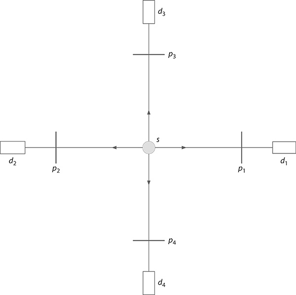
FIGURE 3.8 Experimental configuration of a source emitting two pairs (n = 4) of indistinguishable quanta traveling in four different directions (N = 4) with entangled polarizations. In the theoretical development, it is assumed that all detectors are identical (d₁ = d₂ = d₃ = d₄ = d).

C_{1} = | x 〉_{1} | y 〉_{2} | (ϕ 〉_{3} | (ϕ' 〉_{4} (3.60)

$C_{1} = | x 〉_{1} | y 〉_{2} | (ϕ 〉_{3} | (ϕ' 〉_{4} (3.60)$

C_{2} = | y 〉_{1} | x 〉_{2} | ϕ' 〉_{3} | ϕ 〉_{4} (3.61)

$C_{2} = | y 〉_{1} | x 〉_{2} | ϕ' 〉_{3} | ϕ 〉_{4} (3.61)$

C_{3} = | ϕ 〉_{1} | ϕ' 〉_{2} | x 〉_{3} | y 〉_{4} (3.62)

$C_{3} = | ϕ 〉_{1} | ϕ' 〉_{2} | x 〉_{3} | y 〉_{4} (3.62)$

C_{4} = | ϕ' 〉_{1} | ϕ 〉_{2} | y 〉_{3} | x 〉_{4} (3.63)

$C_{4} = | ϕ' 〉_{1} | ϕ 〉_{2} | y 〉_{3} | x 〉_{4} (3.63)$

The normalization condition

1 = | C_{I} |^{2} + | C_{I I} |^{2} + | C_{I I I} |^{2} + | C_{W} |^{2} (3.64)

$1 = | C_{I} |^{2} + | C_{I I} |^{2} + | C_{I I I} |^{2} + | C_{W} |^{2} (3.64)$

requires that

C_{I} = \frac{1}{\sqrt{4}} (C_{1} + C_{2} + C_{3} + C_{4}) (3.65)

$C_{I} = \frac{1}{\sqrt{4}} (C_{1} + C_{2} + C_{3} + C_{4}) (3.65)$

C_{I I} = \frac{1}{\sqrt{4}} (C_{1} + C_{2} - C_{3} - C_{4}) (3.66)

$C_{I I} = \frac{1}{\sqrt{4}} (C_{1} + C_{2} - C_{3} - C_{4}) (3.66)$

C_{I I I} = \frac{1}{\sqrt{4}} (C_{1} - C_{2} + C_{3} - C_{4}) (3.67)

$C_{I I I} = \frac{1}{\sqrt{4}} (C_{1} - C_{2} + C_{3} - C_{4}) (3.67)$

C_{W} = \frac{1}{\sqrt{4}} (C_{1} - C_{2} - C_{3} + C_{4}) (3.68)

$C_{W} = \frac{1}{\sqrt{4}} (C_{1} - C_{2} - C_{3} + C_{4}) (3.68)$

which lead to the following explicit normalized probability amplitudes

\begin{matrix} | Ψ 〉 & = & \frac{1}{\sqrt{4}} (| x 〉_{1} | y 〉_{2} | ϕ 〉_{3} | ϕ' 〉_{4} + | y 〉_{1} | x 〉_{2} | ϕ' 〉_{3} | ϕ 〉_{4} \\ + | (ϕ 〉_{1} | (ϕ' 〉_{2} | x 〉_{3} | y 〉_{4} + | (ϕ' 〉_{1} | (ϕ 〉_{2} | y 〉_{3} | x 〉_{4}) \end{matrix} (3.69)

$\begin{matrix} | Ψ 〉 & = & \frac{1}{\sqrt{4}} (| x 〉_{1} | y 〉_{2} | ϕ 〉_{3} | ϕ' 〉_{4} + | y 〉_{1} | x 〉_{2} | ϕ' 〉_{3} | ϕ 〉_{4} \\ + | (ϕ 〉_{1} | (ϕ' 〉_{2} | x 〉_{3} | y 〉_{4} + | (ϕ' 〉_{1} | (ϕ 〉_{2} | y 〉_{3} | x 〉_{4}) \end{matrix} (3.69)$

\begin{matrix} | Ψ 〉 & = & \frac{1}{\sqrt{4}} (| x 〉_{1} | y 〉_{2} | (ϕ 〉_{3} | (ϕ' 〉_{4} + | y 〉_{1} | x 〉_{2} | (ϕ' 〉_{3} | (ϕ 〉_{4} \\ - | ϕ 〉_{1} | ϕ' 〉_{2} | x 〉_{3} | y 〉_{4} - | ϕ' 〉_{1} | ϕ 〉_{2} | y 〉_{3} | x 〉_{4}) \end{matrix} (3.70)

$\begin{matrix} | Ψ 〉 & = & \frac{1}{\sqrt{4}} (| x 〉_{1} | y 〉_{2} | (ϕ 〉_{3} | (ϕ' 〉_{4} + | y 〉_{1} | x 〉_{2} | (ϕ' 〉_{3} | (ϕ 〉_{4} \\ - | ϕ 〉_{1} | ϕ' 〉_{2} | x 〉_{3} | y 〉_{4} - | ϕ' 〉_{1} | ϕ 〉_{2} | y 〉_{3} | x 〉_{4}) \end{matrix} (3.70)$

\begin{matrix} | Ψ 〉 & = & \frac{1}{\sqrt{4}} (| x 〉_{1} | y 〉_{2} | (ϕ 〉_{3} | (ϕ' 〉_{4} - | y 〉_{1} | x 〉_{2} | (ϕ' 〉_{3} | (ϕ 〉_{4} \\ + | ϕ 〉_{1} | ϕ' 〉_{2} | x 〉_{3} | y 〉_{4} - | ϕ' 〉_{1} | ϕ 〉_{2} | y 〉_{3} | x 〉_{4}) \end{matrix} (3.71)

$\begin{matrix} | Ψ 〉 & = & \frac{1}{\sqrt{4}} (| x 〉_{1} | y 〉_{2} | (ϕ 〉_{3} | (ϕ' 〉_{4} - | y 〉_{1} | x 〉_{2} | (ϕ' 〉_{3} | (ϕ 〉_{4} \\ + | ϕ 〉_{1} | ϕ' 〉_{2} | x 〉_{3} | y 〉_{4} - | ϕ' 〉_{1} | ϕ 〉_{2} | y 〉_{3} | x 〉_{4}) \end{matrix} (3.71)$

\begin{matrix} | Ψ 〉 & = & \frac{1}{\sqrt{4}} (| x 〉_{1} | y 〉_{2} | ϕ 〉_{3} | ϕ' 〉_{4} - | y 〉_{1} | x 〉_{2} | ϕ' 〉_{3} | ϕ 〉_{4} \\ - | (ϕ 〉_{1} | (ϕ' 〉_{2} | x 〉_{3} | y 〉_{4} + | (ϕ' 〉_{1} | (ϕ 〉_{2} | y 〉_{3} | x 〉_{4}) \end{matrix} (3.72)

$\begin{matrix} | Ψ 〉 & = & \frac{1}{\sqrt{4}} (| x 〉_{1} | y 〉_{2} | ϕ 〉_{3} | ϕ' 〉_{4} - | y 〉_{1} | x 〉_{2} | ϕ' 〉_{3} | ϕ 〉_{4} \\ - | (ϕ 〉_{1} | (ϕ' 〉_{2} | x 〉_{3} | y 〉_{4} + | (ϕ' 〉_{1} | (ϕ 〉_{2} | y 〉_{3} | x 〉_{4}) \end{matrix} (3.72)$

This is a complete symmetrical configuration where the number of path alternatives (N = 4) is matched by the number of particles (n = 4), which corresponds to two pairs of particles propagating via two pairs of alternative paths. Once this mechanics is established, one can readily extend the multiparticle probability amplitude to other similar higher symmetrical configurations.

Problems

3.1 Calculate the diffraction-limited beam divergence at FWHM for (1) a laser beam with a w = 100 μm radius at λ = 590 nm and (2) a laser beam with a w = 500 μm radius at λ = 590 nm.

3.2 Repeat the calculations of Problem 3.1 for λ = 308 nm. Comment.

3.3 Calculate the single-pass dispersive cavity linewidth for a high-power tunable laser yielding a diffraction-limited beam divergence, w = 100 μm in radius, at λ = 590 nm. Assume that an appropriate beam expander illuminates a 3300 lines/mm grating deployed in the first order. The grating has a 50 mm length perpendicular to the grooves.

3.4 (a) For a high-power pulsed laser delivering a Δν ≈ 350 MHz laser line-width, estimate its shortest possible pulse width at FWHM. (b) For a laser emitting Δt ≈ 10 fs pulses, estimate its broadest possible spectral width in nanometers centered around λ = 600 nm.

3.5 Show that Equation 3.34 follows from Equation 3.33.

3.6 Estimate the angular resolution of a single 8.2 m diameter telescope at λ = 500 m.

3.7 Write explicit normalized probability amplitudes for N = 3 propagation channels and n = 6 quanta, that is, three pairs of photons with entangled polarizations.

..................Content has been hidden....................

You can't read the all page of ebook, please click here login for view all page.

Table of Contents for
Chapter 3 The Uncertainty Principle in Optics

3

The Uncertainty Principle in Optics

3.1 Approximate Derivation of the Uncertainty Principle

3.1.1 The Wave Character of Particles

3.1.2 The Diffraction Identity and the Uncertainty Principle

3.1.3 Alternative Versions of the Uncertainty Principle

3.2 Applications of the Uncertainty Principle in Optics

3.2.1 Beam Divergence

3.2.1.1 Example

3.2.2 Beam Divergence and Astronomy

3.2.2.1 Laser Guide Star

3.2.2.2 Example

3.3 The Interferometric Equation and the Uncertainty Principle

3.3.1 Quantum Cryptography

3.3.1.1 Example

Problems

Table of Contents for Chapter 3 The Uncertainty Principle in Optics

Create new playlist

Sign In

Sign Up

Table of Contents for
Chapter 3 The Uncertainty Principle in Optics