
6
Laser Beam Propagation Matrices
6.1 Introduction
A powerful approach to characterize and design laser optics systems is the use of beam propagation matrices also known as ray transfer matrices. This is a practical method that applies to the propagation of laser beams with a Gaussian profile. Since most lasers can be designed to yield beams with Gaussian or near-Gaussian profiles, this is a widely applicable method. Laser beams with Gaussian or near-Gaussian spatial distributions result when the laser emission is single transverse mode or TEM00, as explained in Chapter 7.
From a historical perspective, it should be mentioned that propagation matrices in optics have been known for a while. For early references in the subject, the reader is referred to Brouwer (1964), Kogelnik (1979), Siegman (1986), and Wollnik (1987). In this chapter, the basic principles of propagation matrices are outlined and a survey of matrices for various widely applicable optical elements is given. The emphasis is on the application of the method to practical optical systems. In addition, examples of some useful single-pass and multiple-pass calculations are given. Higher order matrices are also considered.
This chapter follows fairly closely the original version, on this subject matter, published in the work of Duarte (2003) while incorporating some improvements and corrections.
6.2 ABCD Propagation Matrices
The basic idea of propagation matrices is that one vector at a given plane is related to a second vector at a different plane via a linear transformation. This transformation is represented by a propagation matrix. This concept is applicable to the characterization of the deviation of a ray or beam of light through either free space or any linear optical media. The rays of light are assumed to be paraxial rays that propagate in proximity and almost parallel to the optical axis (Kogelnik 1979).
To illustrate this idea further consider the propagation of a paraxial ray of light from an original plane to a secondary plane in free space as depicted in Figure 6.1. In this geometry, the displacement distance l lies on the z-axis, which is perpendicular to x. In moving from the original plane to the secondary plane, the ray of light experiences a linear displacement in the x-direction and a very small angular deviation, that is,
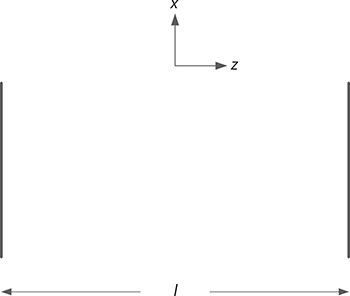
FIGURE 6.1 Geometry for propagation through distance l in free space. The displacement l is along the z-axis that is perpendicular to x.
which in matrix form can be stated as
The resulting 2 × 2 matrix is known as a ray transfer matrix. Here, it should be noted that some authors (Kogelnik 1979; Siegman 1986) use derivatives instead of the angular quantities, that is, dx1/dz = θ1 and dx2/dz = θ2.
For a thin lens, the geometry of propagation is illustrated in Figure 6.2. In this case, there is no displacement in the x-direction and the ray is concentrated, or focused, toward the optical axis so that
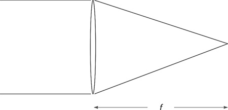
FIGURE 6.2 Thin convex lens.
which in matrix form can be expressed as
In more general terms, the X2 vector is related to the X1 vector by a transfer matrix T known as the ABCD matrix so that
where:
At this stage, it is useful to consider the dimensions of the components involved in these ray transfer matrices: A is a ratio of spatial dimensions, B is an optical length, while C is the reciprocal of an optical length. Consideration of various imaging systems leads to the conclusion that the spatial ratio represented by A is a beam magnification factor (M), whereas D is the reciprocal of such magnification (1/M). More explicitly, the ABCD takes the dimensional format:
These simple observations are very useful to verify the physical validity of newly derived matrices.
6.2.1 Properties of ABCD Matrices
A very useful property of ABCD matrices is that they can be cascaded via matrix multiplication to produce a single overall matrix describing the propagation properties of an optical system. For example, if a linear optical system is composed of N optical elements deployed from left to right, as depicted in Figure 6.3, then the overall transfer matrix is given by the multiplication of the individual matrices in the reverse order, that is,
It is easy to see that the complexity in the form of these product matrices can increase rather rapidly. Thus, it is always useful to remember that any resulting matrix must have the dimensions of Equation 6.9 and a determinant equal to unity, that is,
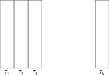
FIGURE 6.3 N optical elements in series.
6.2.2 Survey of ABCD Matrices
In Table 6.1, a number of representative and widely used optical components are represented in ray transfer matrix form. This is done without derivation and using the published literature as reference.
TABLE 6.1
ABCD Ray Transfer Matrices


FIGURE 6.4 Geometry for propagation through distance l in region with refractive index n.
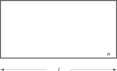
FIGURE 6.5 Slab of material with refractive index n such as an optical plate.

FIGURE 6.6 Concave lens.

FIGURE 6.7 Galilean telescope.
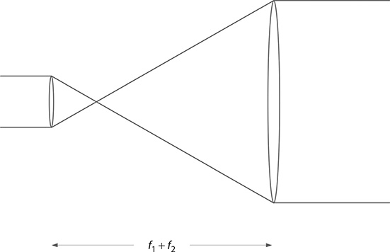
FIGURE 6.8 Astronomical telescope.

FIGURE 6.9 Flat mirror.
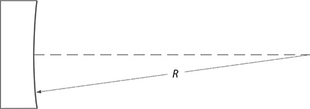
FIGURE 6.10 Curved mirror.
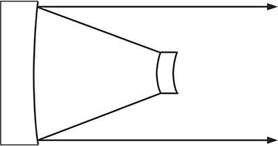
FIGURE 6.11 Reflective telescope of the Cassegrainian class. These reflective configurations are widely applied to unstable resonators, which in the far field can yield a near-TEM00 laser beam profile.
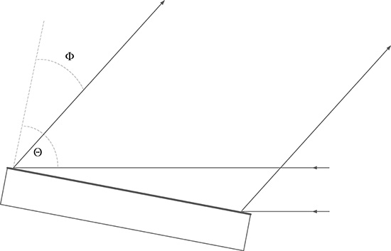
FIGURE 6.12 Generalized flat reflection grating.
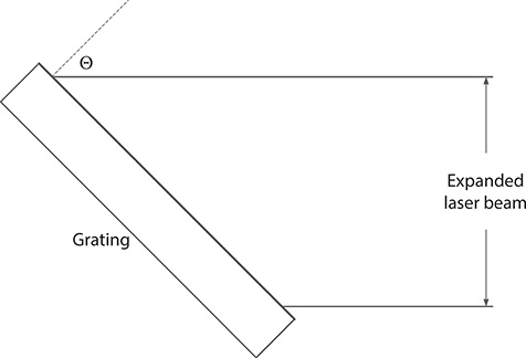
FIGURE 6.13 Flat reflection grating in Littrow configuration.

FIGURE 6.14 Single prism.

FIGURE 6.15 Multiple-prism beam expander.
6.2.3 The Astronomical Telescope
The astronomical telescope (Figure 6.8) is composed of an input lens with focal length f1, an intra lens distance L, and an output lens with focal lens f2. Following Equation 6.10, the matrix multiplication proceeds as follows:
Note that here and further, for notational succinctness, the left-hand side of the equation, that is, the ABCD matrix, is abstracted. For a well-adjusted telescope, where
the transfer matrix becomes
which is the matrix given in Table 6.1. Defining
this matrix can be restated as
For this matrix, it can be easily verified that the condition |AD −BC| = 1 holds.
6.2.4 A Single Prism in Space
For a right-angle prism, with orthogonal beam exit, preceded by a distance L1 and followed by a distance L2, as shown in Figure 6.16, the matrix multiplication becomes
where:
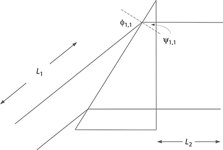
FIGURE 6.16 Single prism preceded by a distance L1 and followed by a distance L2.
Thus, the transfer matrix becomes
which can be restated as
where:
which is the optical length of the system. Notice that both L1 and L2 are modified by the dimensionless beam magnification factor k, whereas l is divided by the dimensionless quantity nk.
6.2.5 Multiple-Prism Beam Expanders
For a generalized multiple-prism array, as illustrated in Figure 6.17, the ray transfer matrix is given by (Duarte 1989, 1991)

FIGURE 6.17 Generalized multiple-prism array (a) Describes an additive configuration and (b) a compensating configuration.
where:
and
For a straightforward multiple-prism beam expander with orthogonal beam exit, cos ψ2,j = 0 and k2,j = 0, so that the equations reduce to
where:
For a single prism, these equations reduce further to M1 = k1,1 and B = l/(k1,1n), which is the result for the single prism given in Table 6.1.
6.2.6 Telescopes in Series
For some applications, it is necessary to propagate TEM00 laser beams through optical systems including telescopes in series as illustrated in Figure 6.18. For a series comprising a telescope followed by a free-space distance, followed by a second telescope, and so on, the single-pass cumulative matrix is given by
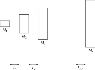
FIGURE 6.18 Series of telescopes separated by a distance Lm.
where:
r is the total number of telescopes
is the B term of the mth telescope
This result applies to a series of well-adjusted Galilean or astronomical telescopes or a series of prismatic telescopes.
6.2.7 Single Return-Pass Beam Divergence
It can be shown (Duarte 1990) that the double-pass or single-return pass divergence in a dispersive laser cavity can be expressed as
where:
which is the Rayleigh length and A and B are the corresponding elements of the ray transfer matrix. The double-pass, or single-return pass, calculation for a narrow-linewidth multiple-prism grating oscillator, illustrated in Figure 6.19, can be performed using the reflection surface of the output coupler mirror as the reference point. For this purpose, the cavity is unfolded about the reflective surface of the output coupler as shown in Figure 6.20. Thus, from the output coupler to the grating and then proceeding from the grating to the output coupler, the matrix multiplication becomes
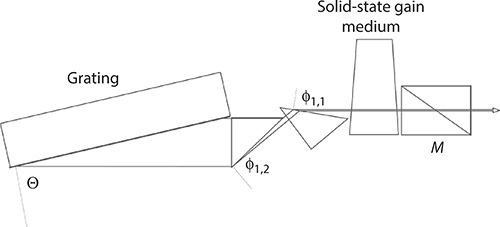
FIGURE 6.19 MPL grating laser oscillator. (Reproduced from Duarte, F.J., Appl. Opt., 38, 6347–6349, 1999. With permission from the Optical Society.)
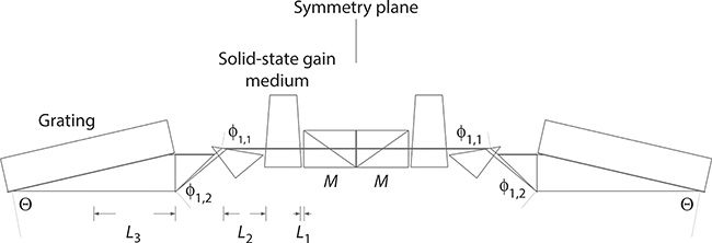
FIGURE 6.20 Unfolded laser cavity for multiple-return-pass analysis. L1 is the intracavity distance between the polarizer output coupler and the gain medium, L2 is the intracavity distance between the gain medium and the multiple-prism expander, and L3 is the intracavity distance between the multiple-prism expander and the diffraction grating.
which reduces to
where:
Multiplication of these matrices in reverse leads to (Duarte et al. 1997)
where:
For an ideal laser gain medium with α ≈ δ ≈ 1, χ ≈ 0, and β ≈ β so that
which imply that the beam divergence will approach its diffraction limit as the optical length of the cavity B increases. This is in accordance with experimental observations.
6.2.8 Multiple Return-Pass Beam Divergence
The multiple-return pass laser linewidth in a dispersive tunable laser oscillator is given by (Duarte 2001)
where:
M is the overall intracavity beam magnification
R is the number of return passes
∇λΘG is the grating dispersion
∇λΦP is the return-pass multiple-prism dispersion
Here, the multiple return-pass beam divergence is given by
where:
AR and BR correspond to cumulative multiple-return pass transfer matrix coefficients
For a multiple-return pass analysis, the cavity is unfolded multiple times and the multiplication described for the single-return pass is performed multiple times. This leads to the following matrix components (Duarte 2001):
and
where:
For a single-return pass,
and
which reduce to Equations 6.37 and 6.38, respectively. Note that by definition A0 = 1 and B0 = 0. For an ideal gain medium, with little or no thermal lensing, α ≈ δ ≈ 1, χ ≈ 0, and β ≈ β, so that
which are the multiple-pass versions of Equations 6.42 and 6.43, respectively. These results mean that, in the absence of thermal lensing, the beam divergence described by Equation 6.47 will decrease toward its diffraction limit as the number of intracavity passes increases. A discussion on the application of these equations to low-divergence narrow-linewidth tunable lasers has been given by Duarte (2001).
6.2.9 Unstable Resonators
The subject of unstable resonators is a vast subject and has been treated in detail by Siegman (1986). Unstable resonators are cavities that are configured with curved mirrors in order to provide intracavity magnification, which in turn provides good transverse-mode discrimination and good far-field beam profiles. In addition to their application as intrinsic resonators, unstable resonators are also widely applied to configure the cavities of forced oscillators that amplify the emission from a master oscillator (see Chapter 7). Here, the discussion is limited to resonators incorporating Cassegrain or Cassegrainian telescopes. These are reflective telescopes, as illustrated in Figure 6.11, which are widely used in the field of astronomy. The double-pass, or single-return-pass ray transfer matrix for a telescope comprising a concave back reflector and a convex exit mirror is given in Table 6.1. The radius of curvature of the mirrors is considered positive if concave toward the resonator. In addition to the transfer matrix, the following relations are useful (Siegman 1986):
and
The condition for lasing in the unstable regime is determined by the inequality:
In addition to traditional unstable resonators of the Cassegrainian type, it should also be mentioned that multiple-prism grating oscillators can also meet the conditions of an unstable resonator when incorporating a gain medium that exhibits thermal lensing (Duarte et al. 1997). However, in the absence of thermal lensing, for an ideal gain medium, α = δ = 1, χ = 0, and β = β, the A and D terms can have a value of unity.
6.3 Higher Order Matrices
The description of optical systems using 3 × 3, 4 × 4, and 6 × 6 matrices has been considered by several authors (Brouwer 1964; Siegman 1986; Wollnik 1987). A more recent description of 4 × 4 matrices, by Kostenbauer (1990), uses the notation:
which can be written as
where the ABCD terms have their usual meaning. For a plane mirror, this matrix becomes
and for a thin concave lens,
For the rth prism, some interesting components of the matrix are given by Duarte (1992):
where:
Going back to the generalized multiple-prism dispersion in its explicit form (Duarte and Piper 1982; Duarte 1988),
and comparing Equation 6.73 with 6.66, we can express the Fr term in shorthand notation as
The explicit Er, Hr, and Ir terms, for a generalized multiple-prism array, are a function of Br. These terms are rather extensive and thus are not included in the text.
Problems
6.1 Derive the ray transfer matrix for the Galilean telescope given in Table 6.1.
6.2 Derive the single-pass ray transfer matrix corresponding to a multiple-prism beam expander, deployed in an additive configuration, comprising four prisms designed for orthogonal beam exit.
6.3 Perform the matrix multiplication for the intracavity single-return pass of the multiple-prism grating tunable laser oscillator depicted in Figure 6.19 that results in Equations 6.37 through 6.40.
6.4 Show that, for a single-pass analysis, Equations 6.51 and 6.52 reduce to the corresponding single-pass A and B terms given by Equations 6.37 and 6.38.
6.5 Use Equations 6.66 and 6.73 to show that the Fr term can be expressed in shorthand as Fr = ∇λϕ2,r (∂λ/∂ν).