
7
Narrow-Linewidth Tunable Laser Oscillators
7.1 Introduction
In this chapter, the basics of interference, the uncertainty principle, polarization, and beam propagation are applied to the design, architecture, and engineering of narrow-linewidth tunable lasers. The principles discussed here apply in general to tunable lasers and are not limited by the type or class of gain media. Thus, the gain media assumed here are generic broadly tunable media in the gas, liquid, or solid state.
A narrow-linewidth tunable laser oscillator is defined as a source of highly coherent continuously tunable laser emission. That is, a laser source that emits highly directional radiation of an extremely pure color. Pure emission in the visible spectrum is defined as having a linewidth narrower than Δν ≈ 3 GHz, which translates approximately into Δλ ≈ 0.0017 nm at λ≈ 510 nm. This criterion is provided by the laser linewidth requirements to excite single vibro-rotational levels in the electronic transition of the iodine molecule at room temperature. Although most of the discussion is oriented toward high-power pulsed tunable lasers, mention of continuous wave (CW) lasers is also made when appropriate.
7.2 Transverse and Longitudinal Modes
A broadband unrefined laser can emit in beams spatially integrating many trans-verse modes and each of these transverse modes can include a multitude of longitudinal modes. A refined, truly coherent, laser should emit in a single transverse mode (TEM00) and, ideally, in a single longitudinal mode (SLM). That orderly, low-entropy emission reaches toward the ideal of monochromatic emission and certainly provides a population of indistinguishable photons.
7.2.1 Transverse Mode Structure
The most straightforward laser cavity comprises a gain medium and two mirrors, as illustrated in Figure 7.1. The physical dimension of the intracavity aperture relative to the separation of mirrors, or cavity length, determines the number of transverse electromagnetic modes. The narrower the width of the intracavity aperture and the longer the cavity length, the lower the number of transverse modes. The single-pass transverse mode structure in one dimension can be characterized using the generalized interferometric equation introduced in Chapter 2 (Duarte 1991a, 1993b)

FIGURE 7.1 Mirror–mirror laser cavity. The physical dimensions of the intracavity aperture relative to the cavity length determine the number of transverse modes.
and in two dimensions using (Duarte 1995b)
In addition, a useful tool to determine the number of transverse modes is the Fresnel number (Siegman 1986):
The single-pass approximation to estimate the transverse mode structure assumes that in a laser with a given cavity length most of the emission generated next to the output coupler mirror is in the form of spontaneous emission and thus highly divergent. Thus, only the emission generated at the opposite end of the cavity and that propagates via an intracavity length L contributes to the initial transverse mode structure.
In order to illustrate the use of these equations, let us consider a hypothetical laser with a 10 cm cavity emitting at λ≈ 590 nm incorporating a 2w = 2 mm-wide one-dimensional aperture. Using Equation 7.1, the intensity distribution of the emission is calculated as shown in Figure 7.2. Each ripple represents a transverse mode. An estimate of this number can be obtained by counting the ripples in Figure 7.2, which yields an approximate number of 17. This number of ripples should be compared with the Fresnel number, which is NF = 16.94.
For the same wavelength, λ≈ 590 nm and a cavity length of L = 10 cm, reducing the dimensions of the intracavity aperture to 2w = 250 μm, yields NF ≈ 026. For such dimensions, the calculated intensity distribution, using Equation 7.1, is given in Figure 7.3. The distribution in Figure 7.3 indicates that most of the emission intensity is contained in a central near-Gaussian distribution, which is the case in practice since the secondary modes can be absent due to cavity losses.
In practice, the spatial distribution of the emission for tunable lasers with the above cavity length-to-intracavity aperture ratio (100,000:125), at visible wavelengths λ ≈ 590 nm, is a near-Gaussian distribution characteristic of what is known as single transverse mode, or TEM00, emission. Additional examples of the beneficial effect derived from the combination of long cavity lengths and narrow intracavity apertures are found in CW lasers, emitting via atomic transitions, that typically yield TEM00 emission. Examples of such coherent sources are the He–Ne, He–Cd, and He–Zn lasers.
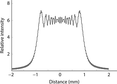
FIGURE 7.2 Cross section of diffraction distribution corresponding to a large number of transverse modes. Here, w = 1.5 mm, L = 10 cm, λ = 632.82 nm, and the Fresnel number becomes NF ≈ 35.56.

FIGURE 7.3 Cross section of diffraction distribution corresponding to a near-TEM00 corresponding to w = 250 μm, L = 40 cm, and λ = 632.82 nm, so that NF ≈ 0.25.
The concept of mode matching in optically pumped laser systems refers to adjusting the dimensions of the excitation laser beam, via optical focusing, to sustain TEM00 emission in the secondary or optically pumped laser. As just explained, these dimensions depend on the necessary cavity length-to-intracavity aperture ratio dictated by the interferometric equation. Reducing the transverse mode distribution to TEM00 emission is the first step in the design of narrow-linewidth tunable lasers. The task of the designer consists in achieving TEM00 emission in the shortest possible cavity length.
7.2.2 Longitudinal Mode Emission
Once TEM00 emission has been established, the task consists in controlling the number of longitudinal modes in the cavity. In a laser with cavity length L, the longitudinal mode spacing, in the frequency domain, is given by (see Chapter 3)
and the number of longitudinal modes NLM is given by
where:
Δν is the measured laser linewidth
Thus, for a laser with a 30 cm cavity length and a measured linewidth of Δν = 3 GHz, the number of longitudinal modes becomes NLM ≈ 6. If the cavity length is reduced to 10 cm, then the number of longitudinal modes is reduced to NLM ≈ 2 and the emission would be called double-longitudinal-mode (DLM) emission. If the cavity length is reduced to 5 cm, then NLM ≈ 1 and the laser is said to be undergoing SLM oscillation. These simple examples highlight the advantages of compact cavity designs, provided the active medium can sustain the gain to overcome threshold.
An alternative to reducing the cavity, and still achieving SLM emission, is to optimize the beam divergence and to increase the intracavity dispersion to yield a narrower cavity linewidth that would restrict oscillation to the SLM regime. In this context, the linewidth
is converted to Δν using the identity
and applying the criterion
to guide the design of the dispersive oscillator.
Multiple-longitudinal-mode emission appears complex and chaotic in both the frequency and temporal domains. DLM and SLM emission can be characterized in the frequency domain using Fabry–Pérot interferometry or in the temporal domain by observing the shape of the temporal pulse. In the case of DLM emission, the interferometric rings appear to be double. In the temporal domain, mode beating is still observed when the intensity ratio of the primary to the secondary mode is 100:1 or even higher. Mode beating of two longitudinal modes, as illustrated in Figure 7.4, can be characterized using a simple wave representation (Pacala et al. 1984) where each mode of amplitudes E1 and E2, with frequencies ω1 and ω2, combine to produce a resulting field
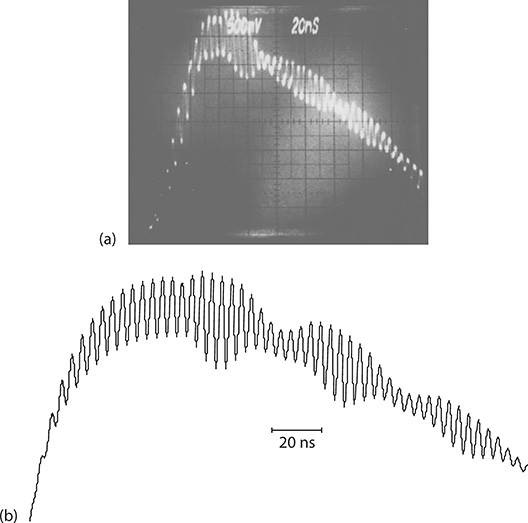
FIGURE 7.4 Mode beating resulting from DLM oscillation. (a) Measured temporal pulse. (b) Calculated temporal pulse assuming interference between the two longitudinal modes. (Reproduced from Duarte, F.J., et al., Appl. Opt., 27, 843–846, 1988. With permission from the Optical Society.)
For incidence at z = 0 on a square-law temporal detector, the intensity can be expressed as
Detectors in the nanosecond regime respond only to the first and last terms of this equation so that the equation can be approximated by
Using this approximation and a non-Gaussian temporal representation, derived from experimental data, for the amplitudes of the form
a calculated version of the experimental waveform exhibiting mode beating can be obtained as shown in Figure 7.4b. For this particular dispersive oscillator lasing in a DLM, the ratio of frequency jitter δω to cavity mode spacing Δω ≈ (ω1 - ω2) was represented by a sinusoidal function at 20 MHz. The initial mode intensity ratio is 200:1 (Duarte et al. 1988; Duarte 1990a).
In the case of SLM emission, the Fabry–Pérot interferometric rings appear singular and well defined (see Figure 7.5). In this case, mode beating in the temporal domain is absent and the pulses assume a smooth near-Gaussian distribution (see Figure 7.6). These results were obtained in an optimized solid-state multiple-prism grating dye laser oscillator for which the limit derived from the uncertainty principle, Δν Δt ≈ 1, is approached (Duarte 1999).
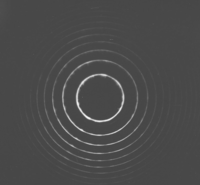
FIGURE 7.5 Fabry–Pérot interferogram corresponding to SLM emission at Δν ≈ 350 MHz. (Reproduced from Duarte, F.J., Appl. Opt., 38, 6347–6349, 1999. With permission from the Optical Society.)
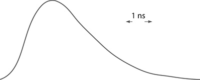
FIGURE 7.6 Near-Gaussian temporal pulse corresponding to SLM emission. The temporal scale is 1 ns/div. (Reproduced from Duarte, F.J., Appl. Opt., 38, 6347–6349, 1999. With permission from the Optical Society.)
7.3 Tunable Laser Oscillator Architectures
Tunable laser oscillators can be configured in a variety of cavity designs. Here, a brief survey of these alternatives is presented. In general, these cavity architectures can be classified into tunable laser oscillators without intracavity beam expansion and tunable laser oscillators with intracavity beam expansion (Duarte 1991a). Further, each of these classes can be divided into open and closed cavity designs (Duarte and Piper 1980). It is assumed that oscillators considered in this section are designed to yield narrow-linewidth emission. The architectures are relevant to a variety of tunable gain media and are applicable to both CW and pulsed lasers.
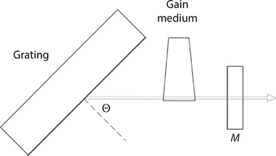
FIGURE 7.7 Grating-mirror tunable laser cavity.
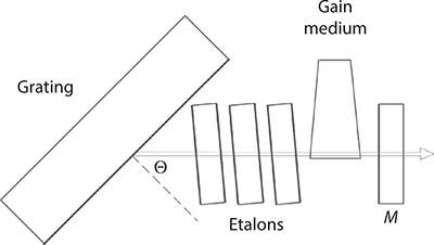
FIGURE 7.8 Grating-mirror laser cavity incorporating intracavity etalons.
7.3.1 Tunable Laser Oscillators Without Intracavity Beam Expansion
Tunable laser oscillators without intracavity beam expansion are those laser resonators in which the intrinsic narrow beam waist at the gain region is not expanded using intracavity optics. The most basic of tunable laser designs is that incorporating an output coupler mirror and a tuning grating in Littrow configuration as illustrated in Figure 7.7. Tuning is accomplished by slight rotation of the grating. This cavity configuration will yield relatively broad tunable emission in a short pulsed laser, such a high-power pulsed dye laser, but could emit fairly narrow emission if applied to a CW semiconductor laser. A refinement of this cavity consists in inserting one or more intracavity etalons to further narrow the emission wavelength as illustrated in Figure 7.8. Such multiple-etalon grating cavity could yield very narrow pulsed emission, down to the SLM regime, in high-power pulsed lasers. The introduction of the etalons provides further avenues of wavelength tuning. The main disadvantage of this class of resonators, in the pulsed regime is the very high intracavity power flux that can induce optical damage in the grating and the coating of the etalons.
An important configuration in the tunable laser oscillators without intracavity beam expansion class, which employs only the natural divergence of the intracavity beam for total illumination of the diffractive element, is the grazing-incidence grating design (Shoshan et al. 1977; Littman and Metcalf 1978). In these lasers, the grating is deployed at a high angle of incidence. The diffracted beam is subsequently reflected back toward the grating by the tuning mirror. A variation on this design is the replacement of the tuning mirror by a grating deployed in Littrow configuration (Littman 1978). This cavity has been configured as a open cavity, as shown in Figure 7.9a, or as a closed cavity, as shown in Figure 7.9b. A further alternative is the inclusion of an intracavity etalon (Saikan 1978) for further linewidth narrowing. Grazing-incidence grating cavities have the advantage of being fairly compact and are widely used in both the pulsed regime and the CW regime. A limitation of these cavities is the relatively high losses associated with the deployment of the diffraction grating at a high angle of incidence as illustrated in Figure 7.10 (Duarte and Piper 1981).
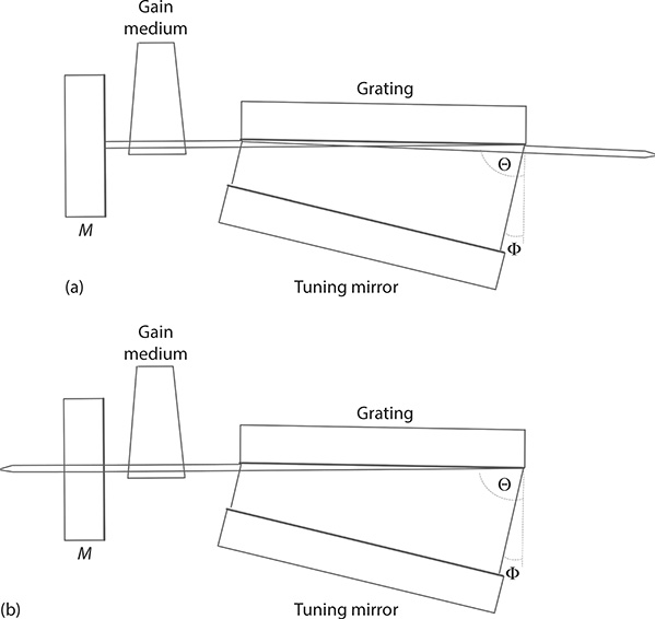
FIGURE 7.9 Grazing-incidence grating cavities: (a) open cavity; (b) closed cavity.
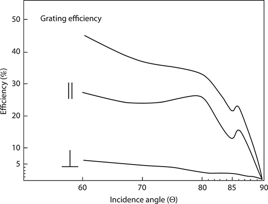
FIGURE 7.10 Grating efficiency curve as a function of angle of incidence at λ = 632.82 nm. (Reproduced from Duarte, F.J., and Piper, J.A., Appl. Opt., 20, 2113–2116, 1981. With permission from the Optical Society.)
For tunable laser oscillators without intracavity beam expansion, and in the absence of intracavity etalons, the cavity linewidth equation takes the fairly simple form
where:
∇λΘG is the grating dispersion either in Littrow configuration
or in grazing-incidence configuration
where the multiple-return-pass beam divergence ΔθR is given by
and the appropriate propagation terms can be calculated according to the optical architecture of the cavity as described in Chapter 6. In Equations 7.13 and 7.18, R refers to the number of intracavity return passes.
For a simple mirror-grating cavity, as illustrated on Figure 7.7, and a single return pass (R = 1), Equation 7.13 reduces to
which provides an estimate of the dispersive linewidth derived from the dispersion of the grating. For a tunable oscillator incorporating a diffraction grating, and an intra-cavity etalon as outlined in Figure 7.8, the dispersive linewidth Δλ can be used via its frequency domain version given by Equation 7.7, that is, Δν, to guide the design of the intracavity etalon with a free spectral range (FSR) is given by (Born and Wolf 1999)
where:
n is the refractive index of the etalon’s material
le is the distance between the reflective surfaces
The expression for the FSR has its origin in Δν = c/Δx as discussed in Chapter 3.
The minimum resolvable linewidth, or resulting laser linewidth, obtainable from the etalon is given by
where:
ℱ is the effective finesse of the etalon
The finesse of the etalon is a function of the flatness of the surfaces (often in the λ/100−λ/50 range), the dimensions of the aperture, and the reflectivity of the surfaces. The effective finesse is given by (Meaburn 1976)
where:
ℱR, ℱF, and ℱA are the reflective, flatness, and aperture finesses, respectively
The reflective finesse is given by (Born and Wolf 1999)
where:
ℛ is the reflectivity of the surface
Further details on Fabry–Pérot etalons are given in Chapter 11.
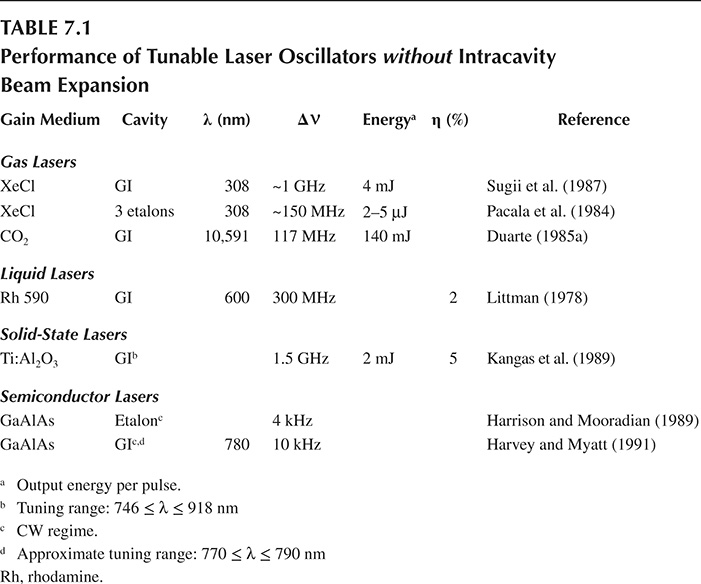
Multiple-etalon systems are described in detail in the literature (Maeda et al. 1975; Pacala et al. 1984). As implied earlier, these multiple-etalon assemblies are designed so that the FSR of the etalon to be introduced is compatible with the measured laser linewidth attained with the previous etalon or etalons. Although this is a very effective avenue to achieve fairly narrow linewidths, the issue of optical damage, due to high intracavity power densities, does introduce limitations. The performance of representative tunable laser oscillators without intracavity beam expansion is summarized in Table 7.1.
TABLE 7.1
Performance of Tunable Laser Oscillators without Intracavity Beam Expansion
7.3.2 Tunable Laser Oscillators With Intracavity Beam Expansion
Equation 7.6 indicates that a key principle in achieving narrow-linewidth emission consists in augmenting the intrinsic intracavity dispersion provided by the diffraction grating. This is accomplished by the total illumination of the diffraction surface of the tuning element. In the case of the grazing-incidence grating cavities, this is done by deploying the grating at a high angle of incidence; however, this can be associated with very low diffraction efficiencies. An alternative method is to illuminate the diffractive element via intracavity beam expansion. Tunable laser oscillators with intracavity beam expansion are divided into two subclasses: those using two-dimensional beam expansion and those using one-dimensional beam expansion.
Initially, intracavity beam expansion was accomplished utilizing two-dimensional beam expansion and a diffraction grating deployed in Littrow configuration as illustrated in Figure 7.11 (Hänsch 1972). Two-dimensional beam expansion has also been demonstrated using reflection telescopes (Beiting and Smith 1979). Transmission telescopes can be either of the Galilean or astronomical class, whereas the reflection telescope can be of the Cassegrainian type (see Chapter 6). The main advantage of this approach is the significant reduction of intracavity energy incident on the tuning grating, thus vastly reducing the risk of optical damage. The main disadvantages of the two-dimensional intracavity beam expansion is the requirement of expensive circular diffraction gratings, a relatively difficult alignment process, and the need for long cavities that incorporate thermal dependence consequences. Since the telescopes mentioned here can provide low dispersion, the cavity linewidth equation reduces to
where:
∇λΘG is the grating dispersion in either Littrow or grazing-incidence configuration, as given in Equations 7.14 through 7.17, and the multiple-return-pass beam divergence ΔθR is given by Equation 7.18.
Certainly, it should be indicated that for a single return pass (R = 1), Equation 7.23 assumes the form of expression introduced by Hänsch (1972):
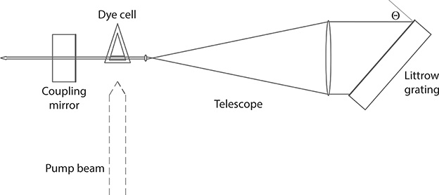
FIGURE 7.11 Two-dimensional transmission telescope Littrow grating laser cavity. This class of telescopic cavity was first introduced by Hänsch.
One-dimensional intracavity beam expansion uses multiple-prism beam expanders rather than conventional telescopes to perform the beam expansion. Multiple-prism grating tunable laser oscillators are classified as multiple-prism Littrow (MPL) grating laser oscillators (Kasuya et al. 1978; Klauminzer 1978; Wyatt 1978; Duarte and Piper 1980) and hybrid multiple-prism grazing-incidence (HMPGI) grating laser oscillators (Duarte and Piper 1981, 1984a). MPL and HMPGI grating laser oscillators are depicted in Figures 7.12 through 7.14. Both of these oscillator subclasses belong to the closed cavity class.
In these laser oscillators, the intracavity beam expansion is one dimensional, thus facilitating the alignment process significantly. In addition, the requirements of the dimensions of the diffraction grating, perpendicular to the plane of incidence, are reduced significantly. Another advantage is compactness since these high-power tunable laser oscillators can be configured in architectures requiring cavity lengths in the 50–100 mm range.
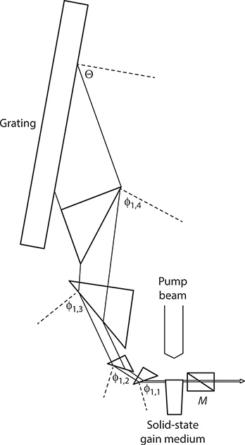
FIGURE 7.12 Long pulse MPL grating solid-state organic dye laser oscillator incorporating a (+, +, +, -) compensating multiple-prism configuration. Laser linewidth is Δν ≈ 650 MHz at a pulse length of Δt ≈ 105 ns. (Reproduced from Duarte, F.J., et al., Appl. Opt., 37, 3987– 3989, 1998. With permission from the Optical Society.)
The solid-state organic MPL grating oscillator depicted in Figure 7.12 incorporates a compensating (+, +, +, -) multiple-prism configurations with M ≈ 90 yielding near-zero prismatic dispersion at λ ≈ 590 nm. The laser linewidth was measured at Δν ≈ 650 MHz for a pulse length of Δt ≈ 105 ns (Duarte et al. 1998). This type of oscillator configuration often uses rather large intracavity beam expansion factors, which in practice can be in the 100 ≤M ≤ 200 range. Oscillator designs with multiple-prism beam magnification factors as high as M ≈ 990 have been described (Shay and Duarte 2009). Further configurational alternatives are discussed in Chapter 4.
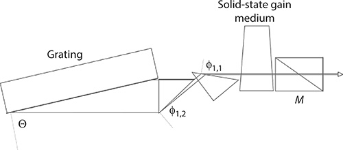
FIGURE 7.13 Optimized compact MPL grating solid-state organic dye laser oscillator. Laser linewidth is Δν ≈ 350 MHz at a pulse length of Δt ≈ 3 ns. (Reproduced from Duarte, F.J., Appl. Opt., 38, 6347–6349, 1999. With permission from the Optical Society.)
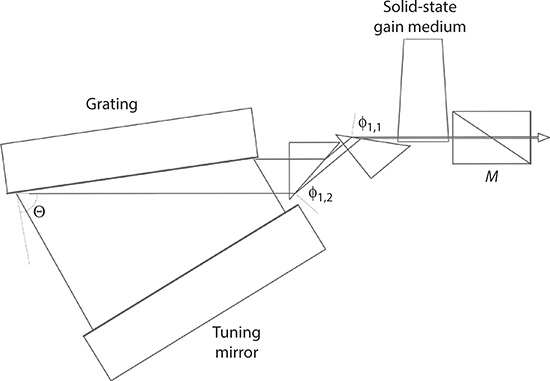
FIGURE 7.14 Solid-state HMPGI grating organic dye laser oscillator. Laser linewidth is Δν ≈ 375 MHz at a pulse length of Δt ≈ 7 ns. (Reprinted from Opt. Laser Technol., 29, Duarte, F.J., Multiple-prism near-grazing-incidence grating solid-state dye laser oscillator, 512–516, Copyright 1997, with permission from Elsevier.)
An optimized dispersive oscillator architecture where a high-density diffraction grating (3300 lines/mm) allows relatively high incidence angles, at Θ≈ 77ख़, in a Littrow configuration is depicted in Figure 7.13 (Duarte 1999). Thus, the required illumination of the diffraction element can proceed with rather modest intracavity beam expansion factors of M ≈ 44. Consequently, the compactness of the cavity is significantly improved. This optimized dispersive solid-state tunable laser oscillator demonstrated laser linewidths down to Δν ≈ 350 MHz, for Δt ≈ 3 ns, which is close to the limit allowed by Heisenberg’s uncertainty principle at a pulse power of ~33 kW (Duarte 1999).
The HMPGI grating oscillator depicted in Figure 7.14 is inherently compact since the grating is deployed at a near-grazing-incidence angle and the required intracavity beam expansion can be provided by a double-prism expander deployed in a compensating configuration to yield M ≈ 30. The difference in efficiency performance between a grating deployed at grazing incidence and a grating deployed at near-grazing incidence can be significant as demonstrated by Duarte and Piper (1981, 1984b) with a clear advantage for the latter. To illustrate this point explicitly, an efficiency curve, as a function of angle of incidence, is provided for a typical diffraction grating in Figure 7.10. Using HMPGI grating oscillator configurations, SLM oscillation at linewidths in the 400 ≤ Δν ≤ 650 MHz have been demonstrated in CVL-pumped tunable liquid organic lasers (Duarte and Piper 1984b) and Δν ≈ 375 MHz in solid-state dye-doped organic polymer gain media (Duarte 1997).
It is interesting to note that most of external semiconductor lasers use the near-grazing-incidence configuration rather than the pure grazing-incidence scheme given the highly divergent beams available from the narrow gain regions of semiconductor lasers. MPL and HMPGI grating oscillator configurations are directly applicable to tunable high-power gas lasers such as excimer lasers and CO2 lasers (Duarte 1985a, 1985b, 1985c) as depicted in Figure 7.15. Using MPL grating configurations, incorporating ZnSe prisms, variable linewidth emission in the 250 ≤ Δν ≤ 650 MHz range was accomplished as a function of M (Duarte 1985b), while an SLM linewidth corresponding to Δν ≈ 107 MHz was measured in a high-power TEA CO2 HMPGI grating oscillator at λ ≈ 10,591 nm (Duarte 1985c).

FIGURE 7.15 (a) MPL and (b) HMPGI grating high-power pulsed CO2 laser oscillators. The prisms are made of ZnSe and the output couplers are made of Ge. (Reproduced from Duarte, F.J., Appl. Opt., 24, 1244–1245, 1985b. With permission from the Optical Society.)
MPL and HMPGI grating oscillators have been shown to inherently yield extremely low levels of amplified spontaneous emission (ASE), which is a very desirable feature in many applications including high-resolution spectroscopy (Duarte and Piper 1980, 1981). The MPL and HMPGI grating oscillators described here (Figures 7.12 through 7.14) incorporate a polarizer output coupler mirror, which is antireflection coated toward the gain medium, whereas its output surface is broadband coated with ~20% reflectivity. The function of this polarizer output coupler mirror is to further suppress the single-pass ASE since the laser emission from these oscillators is intrinsically highly polarized parallel to the plane of incidence. Using these oscillator architectures, ASE levels, as determined by the spectral density ratio ρASE/ρl (Duarte 1990b), are in the 10-7 - 10-6 range (Duarte 1990b, 1997, 1999).
The multiple-return-pass linewidth for a multiple-prism grating oscillator is given by (Duarte and Piper 1984b; Duarte 2001)
where:
∇λΘG is the grating dispersion in either Littrow or grazing-incidence configuration, as given in Equations 7.14 through 7.17, and the multiple-return-pass beam divergence ΔθR is given by Equation 7.18 (see Chapter 4).
In addition to the dispersion of the grating, the multiple-prism must also be considered and is given by (Duarte and Piper 1982a; Duarte 1985c, 1989)
As indicated in Chapter 4, the above equation can be either used to evaluate the return-pass multiple-prism dispersion or applied to design zero-dispersion beam expanders at any given wavelength. In the latter case, λΦP ≈ 0 and Equation 7.25 reduces to Equation 7.23. As described in Chapter 5, the transmission efficiency of the multiple-prism beam expander can be quantified using
and
where:
L1,m, and L2,m, represent the losses at the incidence and exit surfaces of the mth prism, respectively
ℛ1,m, and ℛ2,m, are the respective Fresnel reflection factors given in Chapter 5
The performance of tunable laser oscillators with intracavity beam expansion is summarized in Table 7.2.
TABLE 7.2
Performance of Tunable Laser Oscillators with Intracavity Beam Expansion

7.3.3 Widely Tunable Narrow-Linewidth External Cavity Semiconductor Lasers
The external cavity semiconductor laser (ECSL) has become widely used in a number of contemporaneous applications including laser cooling and Bose–Einstein condensation. Central to the attractiveness of ECSLs is their tunability, narrow- linewidth characteristics, stability, compactness, and low cost. Two of the most popular external cavity configurations belong to the open cavity class in the form of a Littrow grating cavity design (Wieman and Hollberg 1991) and a grazing-incidence grating design (Harvey and Myatt 1991). The adoption of open cavity designs appears to have resulted from a need to adapt to the availability of commercial semiconductor lasers with one end of the cavity sealed from access.
The advantages of closed cavity tunable laser oscillators, over open cavity alternatives, in the pulsed high-power domain, were outlined by Duarte and Piper (1980, 1981). These advantages include significantly reduced optical noise levels and independence from external feedback effects. Albeit the first phenomenon is less pronounced, in semiconductor lasers, the second observation still applies. Moreover, in ECSLs incorporating open Littrow grating configurations, the diffracted beam is directed back to the gain region, while the output is coupled via the reflection losses of the grating. This means that as the wavelength is tuned, the direction of the output beam changes. Thus, additional external optics is required for beam correction (Hawthorn et al. 2001). In ECSLs incorporating open grazing-incidence configuration, tighter boundaries for thermal stability are required (Laurila et al. 2002).
This is interesting given the fact that the closed cavity ECSLs preceded the open cavity alternatives (Voumard 1977; Fleming and Mooradian 1981; Belenov et al. 1983). The main difference is that closed cavity ECSLs require access to both ends of the gain region. Ideally, both ends of the gain region should be antireflection coated as indicated by Fleming and Mooradian (1981) so that the characteristics of the emission are entirely controlled by the external cavity as illustrated in Figure 7.16 (Duarte 1993a). Alternatively, at least one of the cavity ends should be antireflection coated. When this is the case, the frequency-selective elements are deployed next to the antireflection end of the gain region, while the laser output is coupled from the partially reflective extreme (Notomi et al. 1990).
Perhaps, one of the most thoroughly engineered ECSLs to date is that reported by Zorabedian (1992), which was inspired on a closed cavity MPL grating design. Zorabedian reports on a laser linewidth of Δν = 100 kHz sustainable over a 60 nm tuning range, with a side-mode suppression ratio of 70 dB (Zorabedian 1992).
The closed cavity approach has also been demonstrated in the form of a cavity incorporating a transmission Littrow grating (Laurila et al. 2002). These authors report laser linewidths of Δν ≈ 4 MHz over a tuning range of 12 nm centered at λ = 646 nm. The laser beam has an elliptical profile of 8 mm × 1.5 mm (Laurila et al. 2002).
Elliptical TEM00 laser beam profiles are typical in semiconductor lasers and they are a result of the rectangular cross section of the gain region. For instance, rectangular dimensions of 4 μm × 1 μm are not uncommon (Fox et al. 1997). One way to produce, intracavity, a circular beam with tunable narrow-linewidth characteristics is to introduce multiple-prism beam expansion prior to illumination of the transmission grating as illustrated in Figure 7.17a. In this design, the gain region is oriented to emit its elliptical beam with the long axis perpendicular to the plane of incidence. The multiple-prism beam expander then elongates the narrow dimension of the beam to yield a circular profile incident on the grating. As in previous oscillator configurations, the beam expansion, which contributes to the line narrowing, takes place at a plane parallel to the plane of incidence (Duarte 2003). A better solution is to use two antireflection ends to the gain region, deploy the gain region so that the long axis of the beam is perpendicular to the plane of incidence, and provide a large multiple-prism beam expansion prior to the illumination of the diffraction grating deployed in Littrow configuration as shown in Figure 7.17b. At the other end of the cavity, only the necessary beam expansion, parallel to the plane of incidence, is provided to yield a circular beam (Duarte 2009).
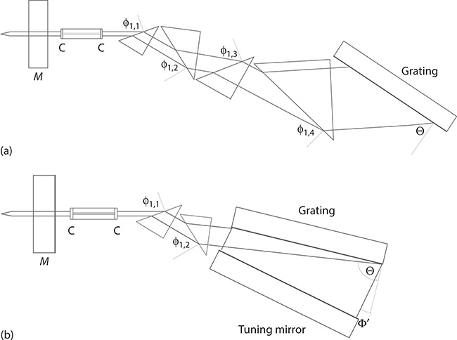
FIGURE 7.16 MPL (a) and HMPGI (b) grating semiconductor laser oscillators. (From Duarte, F. J. (ed.), Broadly tunable external-cavity semiconductor lasers. In Tunable Laser Applications, 2nd edn., CRC Press, New York, Chapter 5, 2009.)
The multiple-prism grating configurations incorporating ZnSe prisms, demonstrated in CO2 lasers (Duarte 1985a, 1985b, 1985c), should be applicable to the design and construction of closed cavity quantum cascade lasers oscillating near λ ≈ 10.6 μm. The performance of tunable external cavity quantum cascade lasers is considered in Chapter 9.
A quantum dot semiconductor laser yielding a linewidth of Δν = 200 KHz, over a tuning range of 1125 ≤ λ ≤ 1288 nm was reported by Nevsky et al. (2008). In this cavity, the initially divergent beam illuminates a collimating lens so that the Littrow grating is illuminated by an expanded intracavity beam. The performance of various tunable semiconductor lasers incorporating intracavity beam expansion is summarized in Table 7.2. Comprehensive reviews on the principles of ECSLs are given by Zorabedian (1995), Duarte (1995a), and Fox et al. (1997).

FIGURE 7.17 (a) MPL transmission grating semiconductor laser oscillator designed to produce circular TEM00 emission. The semiconductor is oriented to emit its elongated beam with the long axis perpendicular to the plane of propagation. Intracavity prismatic beam expansion (parallel to the plane of propagation) renders a nearly circular output beam. (b) MPL grating semiconductor laser oscillator configuration designed to produce circular TEM00 emission. The same expansion strategy is used as in (a) while using a reflection grating in Littrow configuration and beam expansion at both ends of the cavity. The multiple-prism beam expansion illuminating the grating can be as large as necessary to yield very narrow linewidths. (From Duarte, F.J., Tunable Laser Applications, CRC Press, New York, 2009. With permission.)
7.3.4 Distributed Feedback Lasers
A laser architecture that does not belong to either class of resonators previously described, since it does not incorporate mirrors in the optical axis of the emission, is that of the distributed feedback (DFB) laser introduced by Kogelnik and Shank (1971). In these laser configurations, depicted in Figure 7.18, the excitation laser beam is divided into two sub-beams that are recombined at the gain medium where they produce an interference signal. In DFB lasers, feedback is provided by backward Bragg scattering induced by the periodic perturbations of the refractive index at the gain medium. Kogelnik and Shank (1972) have modeled basic gain and spectral features of these lasers using a representation of the scalar wave equation in the form of
and a two counter-propagating wave approach to describe the electric field in the form of
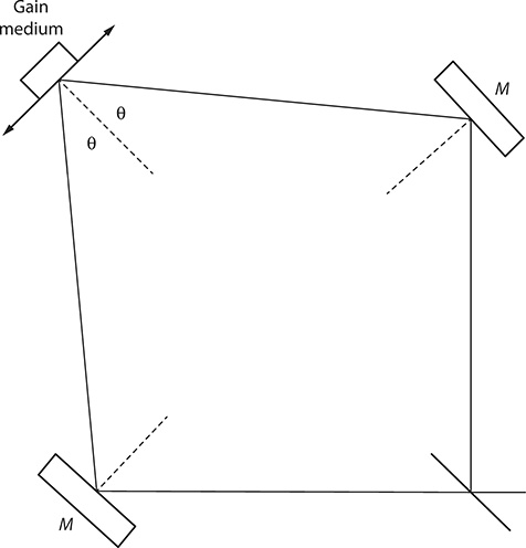
FIGURE 7.18 Generic DFB laser configuration.
where:
z is in the direction of propagation
These authors also assume a periodic spatial variation in the refractive index represented by
where:
κ is related to the fringe spacing Λ by
and the wavelength of oscillation is defined by the Bragg condition (see Section 7.4.4)
The passive linewidth of a DFB laser is given by Bor (1979):
where:
λl is the wavelength of the DBF laser
λp is the wavelength of the pump laser
Δλp is the linewidth of the pump laser
This equation indicates that the linewidth of the DFB laser is determined by the spectral properties of the pump laser. Thus, narrow-linewidth emission in DBF lasers requires a narrow-linewidth pump laser. This is quite different from the lasers using dispersive oscillators whose emission linewidth is independent of the bandwidth of the excitation source.
Tuning DFB lasers can be accomplished by either varying the refractive index of the gain medium or changing Λ. The refractive index can be changed by thermal means or by varying the composition of the gain medium. In the case of DFB dye lasers, it is done by altering the composition of the solvents. For a DFB laser configuration allowing rotation of the mirrors, as shown in Figure 7.18, the fringe separation is given by the first-order grating equation
so that (Shank et al. 1971)
which allows the laser to be tuned by geometrical means.
Given their typical linewidth characteristics, Δν ≈ 45 GHz (Bor 1979), DFB lasers are well-known sources of pulses in the picosecond regime. DFB laser configurations originally applied to liquid dye lasers have also been demonstrated with solid-state dye laser gain media (Wadsworth et al. 1999; Zhu et al. 2000).
In the CW regime, DFB semiconductor lasers have been demonstrated to yield linewidths as low as 2 MHz in the 1.30−1.55 μm wavelength range (Wolf et al. 1991).
7.4 Wavelength Tuning Techniques
Laser oscillators incorporating dispersive, diffractive, and interferometric elements such as prisms, gratings, and etalons are intrinsically tunable. Here, several wavelength tuning techniques based on these elements are described.
7.4.1 Prismatic Tuning Techniques
For a single prism, the exit angle is a function of wavelength as given by (Duarte 1990b)
where:
ζ = sin ϕ1,1 is a constant for a stationary prism
α1 is its apex
angle n(λ, T) is the appropriate material dispersion function
Similarly, the exit angle at the mth prism can be expressed as
where:
ϕ1,m is related geometrically to the exit angle of the preceding prism in the array ϕ2,m−1)
Equation 7.37 highlights the fact that the exit angle at a given prism can be slightly altered by changing the refractive index of the prism, which can be done, for instance, by changing the temperature that exploits the ∂n/∂T of the prism’s material. Also, these equations illustrate the fact that the rays of different wavelengths follow a slightly different geometrical path through the prism sequence.
A purely geometrical tuning approach can be described considering an array of r identical prisms, deployed in a symmetric configuration, and a mirror as shown in Figure 7.19. The cumulative angular displacement at the exit surface of the last prism is augmented according to (Duarte 1990a)
Again this means that a wave front of different wavelengths emerges at a slightly different angle at the exit prism of the array. Thus, depending on the cumulative dispersion, the tuning mirror can only reflect back light within a narrow bandwidth. At a slightly different angular position, the light of a slightly different wavelength is reflected back to the gain region. Using this approach, Strome and Webb (1971) report a tuning range from 571 to 615 nm using a four-prism sequence in a pulsed dye laser.
7.4.2 Diffractive Tuning Techniques
Diffraction gratings are the main tuning elements in narrow-linewidth dispersive laser oscillators. In a cavity incorporating a grating deployed in a grazing-incidence, or near-grazing-incidence, configuration (as illustrated in Figure 7.20), the wavelength is changed by rotating the tuning mirror. Wavelength tuning in this configuration is described by the grating equation:
where:
Θ is the angle of incidence
Φ is the angle of refraction
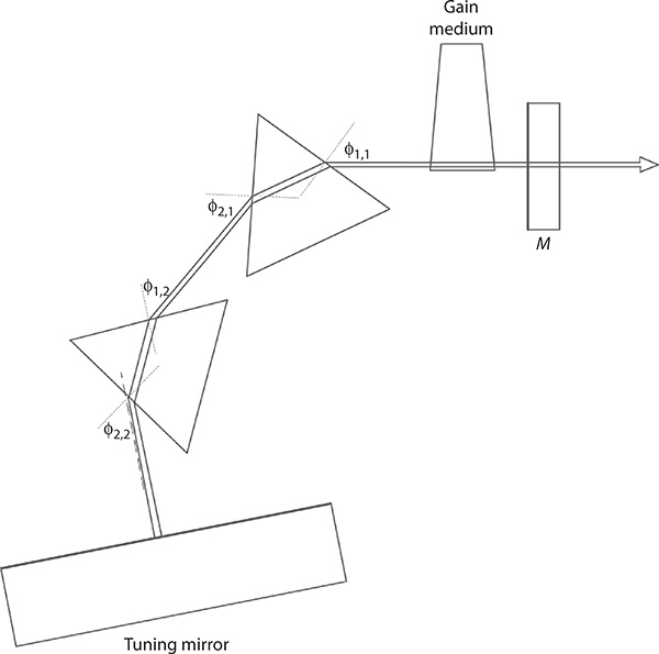
FIGURE 7.19 Multiple-prism tuning.

FIGURE 7.20 Diffraction grating deployed in near-grazing-incidence configuration.
For a fixed angle of incidence, different wavelengths diffract at different angles. Hence, the precise angular position of the tuning mirror determines the wavelength of the radiation that will return to the gain region for further amplification. Geometrically, the tuning is described by Equation 7.40, where m, d, and Θ are kept constant so that λ becomes a function of sin Φ.
For a grating in Littrow configuration, Θ = Φ (see Figure 7.21), and the grating equation becomes
and with m and d being fixed, λ becomes solely a function of sin Θ. Using these simple diffraction techniques, narrow-linewidth dispersive laser oscillators have been smoothly tuned over 50 nm or more (Duarte 1990a, 1999).
Accurate angular displacement of tuning gratings requires the use of high-quality kinematic mounts with 0.1 s of arc or better. For an MPL grating oscillator, a frequency shift of δν ≈ 250 MHz, comparable to the Δν of the dispersive oscillator, requires an angular rotation of δΘ ≈ 10−6 radians at the grating (Duarte et al. 1988).

FIGURE 7.21 Diffraction grating deployed in Littrow configuration. Here, the angle of incidence equals the angle of diffraction (Θ = Φ).
7.4.2.1 Example
In an optimized multiple-prism grating tunable laser oscillator, as illustrated in Figure 7.13, the multiple-prism expander is designed to yield zero dispersion at the central wavelength of emission, in this case λ ≈ 590 nm, and the tuning characteristics of the laser are entirely dominated by the 3300 lines/mm diffraction grating deployed in a Littrow configuration at m = 1. Thus, to tune from λ1 ≈ 590.0000 to λ2 ≈ 590.0004, it is necessary to rotate the diffraction grating by a minute angle determined by λ1 = 2d sin Θ1 and λ2 = d sin Θ2, since m = 1 in Equation 7.41. Substitution by the given quantities, and computation of the angles related to the given wavelengths, yields an angular difference of δΘ ≈ 2.8860 × 10⁻⁶ radians. This is the angular displacement necessary to tune approximately by Δν ≈ 350 MHz, which is the measured linewidth of this multiple-prism grating laser oscillator (Duarte 1999). This example illustrates the functional elegance of this class of high-power pulsed tunable oscillator.
7.4.3 Synchronous Tuning Techniques
As the wavelength of the oscillator is being tuned using a dispersive element such as a diffraction grating, in either grazing-incidence or Littrow configuration, the FSR of the cavity, or the spacing of the longitudinal modes, varies according to
This can lead to abrupt jumps in the longitudinal mode selection, which is also known as mode hopping. One way to suppress this effect is to adjust the cavity length accordingly so that the FSR of the cavity is not altered. This is known as synchronous tuning. In cavities tuned by a grating deployed in Littrow configuration, synchronous tuning can be achieved by synchronizing the position of the output coupler mirror with the rotation of the grating. Although this is a simple principle, its successful practical implementation requires the application of accurate wavelength monitoring and high-precision servomechanisms.
An alternative approach to synchronous wavelength tuning, applicable to SLM lasers, was introduced by Littman (1981) who realized that the cavity length (see Figure 7.22) is an integral number of half wavelengths so that
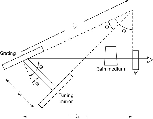
FIGURE 7.22 A synchronous wavelength tuning configuration.
where:
N is the number of longitudinal modes
Comparison of this equation with
indicates that equivalence is achieved if (Littman 1981)
and
Careful selection of the cavity parameters involved in these equations can lead to the establishment of a fairly wide single-mode scanning range. This scheme requires high-precision rotation of the tuning mirror since the mechanical displacement equivalent to half a wavelength can result in mode hopping (Littman 1981).
7.4.4 Bragg Gratings
One further method of wavelength tuning, applicable to ECSLs and fiber lasers, is the use of Bragg gratings (Kogelnik and Shank 1972). In a fiber laser, for instance, a grating can be engraved in the fiber with the grooves perpendicular to the plane of propagation using suitable laser radiation. A Bragg grating can be visualized as a wavelength-selective mirror satisfying the Bragg condition:
where:
n is the refractive index
Λ is the grating period
The linewidth selectivity can be estimated using (see Chapter 3)
with Δ x = 2nd, for propagation in a bulk material of refractive index n, so that
where:
d is the thickness of the grating
The gating period can also be defined as Λ = d/N, where N is the number of planes in the grating. Thus, in terms of explicit grating parameters, the wavelength can expressed as
and the linewidth as
For assessment and comparison purposes, it is useful to restate the interferometric identity in frequency units
or
7.4.5 Interferometric Tuning Techniques
In addition to prismatic and diffractive tuning methods, intracavity etalons provide a further alternative for fine wavelength tuning. According to Born and Wolf (1999), the etalon can be considered as a periodic wavelength filter that satisfies the following condition for maxima:
where:
me is an integer
de is the distance between the reflective surfaces
ψe is the refraction angle that is related to the tilt angle by
n(λ, T) is the refractive index of the substrate of the etalon (see Figure 7.23)
The angular dispersion of the etalon can be written as (Duarte 1990b)
where:
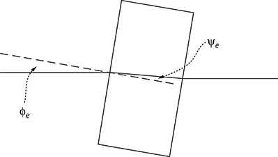
FIGURE 7.23 Solid etalon depicting incidence and refraction angles.
For n = 1, the condition ∇λϕe = ∇λψe arises so that
as given by Schäfer (1990). For the special case of n = 1, it can be shown that the wavelength shift resulting from a displacement in Ie (from ϕe = 0 at O1) is given by (Schäfer 1990)
In addition to angular rotation, an alternative fine-tuning technique exploits the thermal dependence of the refractive index of the etalon’s substrate. Using Equation 7.53, the wavelength difference from λ1 to λ2 corresponding to a change in temperature from T1 to T2 can be written as
which for ψe1 = 0 at λ1 reduces to
For the special case of n(T1) = n(T2) = 1, this equation takes the form of Equation 7.58.
In addition to solid etalons, gas-spaced Fabry–Pérot interferometers can also be used for fine frequency tuning. Meaburn (1976) indicates that the refractive index of the gas can be varied, as a function of pressure, according to
where:
K is a constant related to the intrinsic properties of the gas
ΔP is the pressure gradient applied over the plates of the interferometer
The wavelength shift thus obtained can be expressed as (Meaburn 1976)
This principle was applied by Wallenstein and Hänsch (1974) to vary the frequency of a telescopic dye laser oscillator, including a tilted etalon and a grating mounted in Littrow configuration. According to these authors, the laser frequency changes almost linearly, as a function of pressure, according to
7.4.6 Longitudinal Tuning Techniques for Laser Microcavities
Longitudinal tuning is the result of slight changes in cavity length as illustrated in Figure 7.24. This section is based on the original discussion on longitudinal tuning techniques by Duarte (2003) and refinements made in the work of Duarte (2014).
The principle of longitudinal tuning is based on the interferometric identity
which can also be stated as
Assume that the cavity linewidth Δλ remains constant at two relatively close but different wavelengths as illustrated in Figure 7.25. This is a reasonable assumption for a laser emitting a diffraction-limited beam. Under these circumstances, the spacing of the intracavity modes will change within the transmission window so that

FIGURE 7.24 Longitudinal tuning applicable to laser microcavities. The cavity length L is changed by a minute amount ΔL (see text).
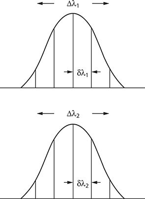
FIGURE 7.25 Dispersive cavity linewidth at two slightly different frequencies. It is assumed that Δλ1 ≈ Δλ2, while the intracavity FSR changes.
or
for Δλ1 ≈ Δλ2,
or
for ΔL = 0, δλ1 ≈ δλ2, and λ1 ≈ λ2. For multilongitudinal mode oscillation, this approach requires counting the number of modes at the two wavelengths. For SLM oscillation, N1 = N2 = 1 and
This equation indicates that tuning, by changing the cavity length, depends directly on the (ΔL/L) ratio. For instance, a tunable dispersive oscillator yielding SLM emission (Δν ≈ 350 MHz) with a cavity length of L = 75 mm (Duarte 1999) can tune its emission wavelength from 590.0000 to 590.0197 nm by increasing its cavity length just by ΔL = 0.005 mm. This wavelength change translates to a frequency shift of δQ ≈ 17 GHz. Given a laser linewidth of Δν ≈ 350 MHz, such change in the cavity length translates into an enormous frequency shift. This implies that the cavity length, and thus the thermal conditions, of such oscillators must be carefully controlled to ensure stability in the frequency domain. For the case of a miniature laser cavity, with a length of 1 mm, tuned with MEMS methods and lasing at 650 nm, the frequency can be tuned in steps of 2.3 GHz by changing the cavity length every 10 nm.
7.4.6.1 Example
Uenishi et al. (1996) reported on experiments using the ΔL/L method to perform wavelength tuning in a MEMS-driven semiconductor laser cavity. In such experiments, they observed wavelength tuning, in the absence of mode hopping, as long as the change in wavelength did not exceed λ2 - λ1 ≈ 1 nm. Using their graphical data for the scan initiated at λ1 ≈ 1547 nm, it is established that ΔL ≈ 0.4 μm, and using L ≈ 305 μm, Equation 7.72 yields λ2 ≈ 1548 nm, which approximately agrees with their observations (Uenishi et al. 1996). In this regard, it should be mentioned that Equation 7.72 was implicitly derived with the assumption of a wavelength scan obeying the condition δλ1 ≈ δλ2. Albeit here, we use the term microcavity, this approach should also apply to cavities in the submicrometer regime or nanocavities.
7.4.7 Birefringent Filters
Birefringence in intracavity wavelength selectivity occurs via the use of birefringent filters (see also Chapter 5). The spatial phase component in the wave equation
for a uniaxial crystal plate can be expressed in more detail as (Born and Wolf 1999)
which can be written as
Maximum transmission, for a single birefringent plate, will occur for values of δ = 2πm (where m = 1, 2, 3, ...) so that, at a transmission maximum designated by λmax,
so that using Δλ ≈ λ2/2xΔn the linewidth becomes
Birefringent filters for wavelength tuning applications are often used in stacks and are known as Lyot filters. The use of a three-plate birefringent filter as an intracavity wavelength selectivity element was described by Johnston and Duarte (2002).
7.5 Polarization Matching
The polarization characteristics of a given tunable laser oscillator depend on the intrinsic polarization of the gain medium, the angle of the laser windows (or emission exit surfaces), the configuration of the dispersive elements, and the diffraction grating. For optimum laser conversion efficiency, it is important to perform a polarization matching of the gain region to that of the optical elements integrating the laser cavity. For the purpose of this discussion, the plane of incidence is as defined in Chapter 5.
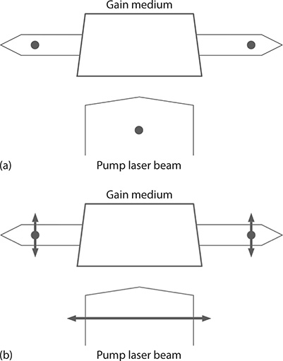
FIGURE 7.26 Polarization preference as explained by Duarte (1990b): (a) An excitation beam polarized perpendicular to the plane of propagation yields emission also polarized perpendicular to the plane of propagation; (b) the same excitation emission polarized parallel to the plane of propagation yields emission, in the same molecular active medium, partially polarized in both directions (see text).
The polarization characteristics of a given gain medium depend on the atomic or molecular composition of such medium. A gain medium such as a laser dye responds differently to different orientations of the polarization of the pump laser (Schäfer 1990). As illustrated in Figure 7.26 (Duarte 1990b), excitation with the pump laser beam polarized perpendicular to the plane of propagation yields single-pass emission, which is also polarized perpendicular to the plane of incidence when using rhodamine 590 molecules, as the gain medium, and the 2P3/2 − 2D5/2 transition of the copper laser (λ = 510.554 nm) as the excitation radiation. However, for excitation parallel to the plane of incidence, the emission is almost unpolarized.
7.6 Design of Efficient Narrow-Linewidth Tunable Laser Oscillators
The design of efficient optically pumped high-power pulsed tunable laser oscillators follows a well-defined series of stages that are outlined in chronological order.
The first opportunity to induce a given polarization is presented in the selection of the angle of the laser windows. Windows deployed at an angle, thus creating a gain region in form of a trapezoid, greatly reduce internal reflections, contribute significantly to reduce optical noise, and facilitate the control of the spectral characteristics by the dispersive optics. The reflection losses for the given components of polarization are given by (Born and Wolf 1999)
For a multiple-prism grating oscillator, the reflection losses at the multiple-prism beam expander are calculated using Equations 7.27 and 7.28. The polarization efficiency response of a typical holographic grating suitable for linewidth narrowing and tuning in dispersive tunable laser oscillators is illustrated in Figure 7.10.
Given that the polarization efficiency response of the grating clearly favors radiation polarized parallel to the plane of incidence, and the fact that the natural deployment of the multiple-prism beam expander (see Figure 7.13) also induces polarization parallel to the plane of incidence, it is logical to deploy the gain medium as illustrated in Figure 7.26, that is, with the windows at an angle, relative to the orthogonal to the optical axis, and the trapezoid parallel to the plane of incidence. As described in Chapter 5, the closer this angle gets to the Brewster angle, the greater the preference for radiation polarized parallel to the plane of incidence. Finally, the orientation of the polarization of the excitation laser should be selected so that the single-pass emission is compatible with the polarization preference of the architecture of the oscillator. In this particular case, the pump laser radiation should be selected to yield unpolarized single-pass emission as shown in Figure 7.26b.
Using the approach described here, Duarte and Piper (1984a) demonstrated SLM emission ~100% polarized parallel to the plane of incidence in a high-pulserepetition-frequency copper laser-pumped dye laser. Polarization matching of the excitation laser to the polarization preference of the multiple-prism grating oscillator yields an increase of 15% in the laser conversion efficiency (Duarte and Piper 1982b). It should be indicated that although a specific example was used to describe the idea of polarization matching, the simple principles described are applicable to any laser system and even to extracavity optics for the efficient transmission of laser radiation.
7.6 Design of Efficient Narrow-Linewidth Tunable Laser Oscillators
The design of efficient optically pumped high-power pulsed tunable laser oscillators follows a well-defined series of stages that are outlined in chronological order.
Select the most efficient pump laser for the given medium. In the case of molecular gain media, the efficiency follows approximately the ratio (Shank 1975):
where:
λe is the emission wavelength
λp is the wavelength of the pump source
In addition to better efficiency, in the case of visible dye lasers, an excitation source with a wavelength close to the emission wavelength enhances significantly the lifetime of the gain medium. Specifically, the lifetime of rhodamine dye solutions using copper vapor laser excitation is vastly superior to the lifetime of the same molecular medium under the excitation of ultraviolet lasers.
Determine the energy density threshold for optical damage of the gain medium.
Select the geometry of the gain medium. A trapezoid geometry is recommended to eliminate internal reflections and thus facilitate the frequency control with the intracavity optics.
Once the approximate cavity length has been determined, select the dimensions of the beam waist (w) at the gain region adequate to yield TEM00 emission. This could be done applying Equations 7.1 through 7.3 or experimentally. An important issue here is not to exceed the energy density threshold for optical damage of the gain medium. For a given cavity length, verify experimentally that TEM00 emission is present.
Select the cavity architecture that best matches the application. Here, issues of compactness, simplicity, and efficiency play an important role.
Select an efficient high-density diffraction grating suitable for the required tuning range. Use Equations 7.14 through 7.17 to determine the dispersion and Equations 7.40 and 7.41 to calculate the tuning range of a given grating.
If intracavity beam expansion is required, select the appropriate method of expansion. For telescopic beam expansion, use the matrix equations in Chapter 6 to design an appropriate two-dimensional beam expander. If a multiple-prism beam expander is selected, use Equation 7.26 to design the multiple-prism array and Equations 7.27 and 7.28 to determine its transmission efficiency. The beam expander selected should have polarization characteristics compatible with those of the diffraction grating.
Perform a return-pass linewidth calculation using Equation 7.25. Adjust the cavity length to satisfy the criterion established in the inequality Δν ≤ δν.
If the dispersion of the cavity is not sufficient to satisfy the criterion in the inequality Δν ≤ δν, either redesign the oscillator to attain a shorter cavity or insert an intracavity etalon. The etalon can be designed using Equations 7.19 through 7.22.
Depending on the optical components integrating the cavity, select the method of wavelength tuning.
Determine the polarization preference of the cavity and compare it to the polarization of the excitation source. Perform polarization matching if necessary.
Determine the ρASE / ρl ratio. If necessary, replace the output coupler mirror by a polarizer output coupler mirror as illustrated in Figure 7.13.
Optimize alignment and measure the conversion efficiency, tuning range, Δθ, and Δλ. If SLM oscillation is not observed, either decrease the cavity length or increase the intracavity dispersion.
7.6.1 Useful Axioms for the Design of Narrow- Linewidth Tunable Laser Oscillators
The design of efficient dispersive narrow-linewidth tunable laser oscillators does benefit from the careful application of a number of well-defined, and specific, rules of physics that can be classified as follows:
The longer the cavity and the narrower the beam waist, the better the beam quality of the laser emission, or
The larger the optical length of the cavity, the lower the beam divergence, or
For diffraction-limited TEM00 emission, the narrower the beam waist w, the larger the beam divergence, or
The larger the beam magnification, the larger the intracavity dispersion, and the narrower the linewidth, or
Also, from the previous axiom, the lower the beam divergence, the narrower the linewidth.
From the second and fourth axioms, the larger the number of intracavity passes, the lower the beam divergence and the narrower the linewidth.
The shorter the cavity, the longer the longitudinal mode spacing, or
These axioms clearly illustrate that some of the design parameters have a competing effect on the overall physics. The task of the designer is to apply these principles in a balanced approach to optimize the beam divergence and linewidth performance in a compact cavity architecture.
7.7 Narrow-Linewidth Oscillator-Amplifiers
The dispersive tunable laser oscillators so far described yield SLM emission at very low levels of ASE. However, for many applications, high energies or high-average powers are required. For that purpose, the exquisite emission from the oscillator must be amplified by one or several amplification stages. A review on this subject, and its literature, is given by Duarte (1990b). Here, the focus will be on the fundamentals and the performance of various representative systems.
7.7.1 Laser-Pumped Narrow-Linewidth Oscillator-Amplifiers
Amplification of coherent optical radiation in laser-excited systems is well illustrated by the configurations developed for dye lasers. Two of the most interesting features of these systems are that amplification is performed in a single pass and that several stages of amplification are often employed. As such, given that lasing in these systems occurs in the nanosecond regime, it is important to synchronize the arrival of the oscillator pulse with the excitation of the amplifier. This is arranged by allowing the excitation geometry to delay the pump pulse as illustrated in Figure 7.27. An additional aspect important to the design of multistage oscillator-amplifier systems is the geometrical matching of the oscillator, or preamplified, beam with the focused excitation laser at the corresponding amplifier stage. This helps to maintain the cumulative ASE at low levels. For optimum efficiency, proper distribution of the pump energy is required with only a fraction (often less than a 5%) of it being used to excite the oscillator. Correct polarization matching is also important.
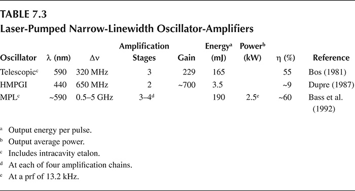
The performances of illustrative multistage oscillator-amplifier laser systems are listed in Table 7.3. Bos (1981) reports 6% efficiency at the oscillator, 20% at the pre-amplifier, and 60% ant the amplifiers. The overall gain factor is about 229. The copper vapor laser-pumped dye laser reported from Lawrence Livermore (Bass et al. 1992) operates at a pulse repetition frequency of 13.2 kHz and comprises several master oscillator (MO) power amplifier (MOPA) chains performing at a 50%–60% overall conversion efficiency. The MOs are of the MPL grating class and incorporate an intra-cavity etalon, and each MOPA chain includes three to four amplifiers in series.
Although most oscillator-amplifiers systems considered here utilize high-performance pulsed MOs, the alternative of semiconductor laser oscillators, lasing in the CW regime, is also available as demonstrated by Farkas and Eden (1993).
These authors used a five-stage dye laser amplification system to produce pulses of 1.2 mJ at 786 nm with Δν = 118 MHz.
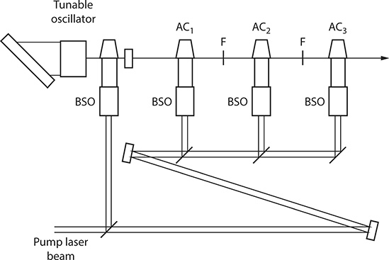
FIGURE 7.27 Multiple-stage single-pass laser amplification.
TABLE 7.3
Laser-Pumped Narrow-Linewidth Oscillator-Amplifiers
7.7.2 Narrow-Linewidth MO Forced Oscillators
The MO is composed of narrow-linewidth dispersive laser oscillators already discussed. The forced oscillator (FO), however, is an amplifier stage comprising a gain region within a resonator as depicted in Figure 7.28. The resonator of the amplifier stage can be an unstable resonator. Several aspects are rather critical to the efficient frequency locking of these configurations. First, the alignment of the MO relative to the FO must be concentric. Second, there are stringent requirements for the timing of the excitation that impose arrival of the MO pulse at the onset of the FO pulse buildup. Efficient frequency locking also occurs. Optimum lasing is achieved when the emission wavelength of the MO is tuned to the central wavelength of the gain spectrum of the FO. The performance of some representative MOFO systems is described in Table 7.4.
TABLE 7.4
Narrow-Linewidth MOFOs
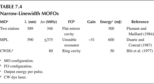
The FO cavity depicted in Figure 7.28 is configured after a Cassegrainian telescope and is cataloged as a confocal unstable resonator of the positive branch (Siegman 1986). Here, the radius of curvature of the large concave mirror is R2, whereas the radius of the small mirror is R1 and has a negative value. The magnification of the resonator is given by (Siegman 1986)
and its length is
As discussed by Siegman (1986), the condition for oscillation in the unstable regime is satisfied by
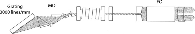
FIGURE 7.28 Master oscillator Forced oscillator laser configuration. (Reproduced from Duarte, F.J., and Conrad, R.W., Appl. Opt., 26, 2567–2571, 1987. With permission from the Optical Society.)
where:
A and D are the matrix elements introduced in Chapter 6
For the resonator depicted in Figure 7.27, R1 = −2 m and R2 = 4 m, so that M = 2, L = 1 m, and the condition for lasing in the unstable regime is satisfied.
In Chapter 6, it is mentioned that narrow-linewidth multiple-prism grating oscillators can lase in the unstable regime in the presence of thermal lensing at the gain medium (Duarte et al. 1997). Finally, although the focus given here is on high-power pulsed lasers in the liquid phase, the principles illustrated apply to lasers in general.
7.8 Discussion
In this section, a concept previously introduced in Section 7.2 is discussed further. Besides the obvious practical significance and advantages of tunable narrow-linewidth laser emission, there is an important physical dimension to this topic. Raw unrefined broadband high-power multiple-transverse-mode emission, with each of those transverse modes containing a multitude of longitudinal modes, is a manifestation of entropy in directed energy. Refining that broadband emission to a TEM00 and then to a SLM is a transparent example of entropy reduction in nature, which is beautifully captured by the cavity linewidth equation:
which tells the designer that to produce very pure narrow-linewidth emission, with a minimum of entropy, the beam divergence must be minimized and the dispersion of the cavity must be augmented. The word dispersion here means the continuous orderly arrangement of wavelengths in the spectrum. High intracavity dispersion leads to the emission of indistinguishable photons in a narrow-linewidth distribution. In other words, intracavity dispersion reduces entropy.
Problems
7.1 For a laser, emitting at λ = 590 nm, with a beam waist of w = 100 μm and a cavity length of 10 cm, calculate the Fresnel number. Comment on the likely beam profile of this laser.
7.2 For a dispersive oscillator lasing with a TEM00 beam profile at λ = 590 nm and a cavity length of 10 cm, calculate the longitudinal mode spacing. Assuming that the calculated single-return-pass dispersive linewidth is Δν = 500 MHz, determine whether this oscillator design is likely to yield an SLM emission, given that the temporal pulse is known to be 5 ns long at full width at half maximum.
7.3 For a dispersive laser oscillator yielding DLM emission with δQ = 1 GHz, design a suitable etalon to restrict oscillation to an SLM. Assume a fairly high-surface finesse and neglect the aperture finesse. Select a suitable reflectivity to allow maximum transmission while restricting oscillation to an SLM.
7.4 For a multiple-prism grating laser oscillator with w = 117 μm and M = 100, calculate the single-return-pass linewidth for a 5 cm grating with 3000 lines/mm. Assume λ = 590 nm, a diffraction-limited laser beam, and that the multiple-prism expander was designed to yield zero dispersion at this wavelength.
7.5 For an optimized tunable laser oscillator with a cavity length of 50 mm and lasing in an SLM at λ = 590 nm, calculate the wavelength shift due to a decrease of 50 μm in cavity length.
7.6 Design, step by step, a multiple-prism grating oscillator capable of yielding an SLM lasing at λ = 590 nm. Assume that a beam waist of w = 100 μm can be attained at the gain region and that a 5 cm grating is available which has 3300 lines/mm. Use a double-prism beam expander and configure it to yield zero dispersion at the given wavelength. Select a cavity length providing a longitudinal mode spacing approximately equal to the return-pass linewidth.