Chapter 8 Nonlinear Optics

Search in book...
Toggle Font Controls
Create new playlist

Name your new playlist

Playlist description (optional)
Sign In

Email address

Password

Forgot Password?

or

Continue with Facebook

Continue with Google
Sign Up

Full Name

Email address

Confirm Email Address

Password

or

Continue with Facebook

Continue with Google

The subject of polarization as related to reflection and transmission in isotropic homogeneous optical media, such as optical glass, was considered via Maxwell’s equations in Chapter 5. Here, we consider the subject of propagation and polarization in crystalline media that gives origin to the subject of nonlinear optics. The brief treatment given here is at an introductory level and designed only to highlight the main features relevant to frequency conversion. For a detailed treatment on the subject of nonlinear optics, the reader is referred to a collection of books on nonlinear optics including Bloembergen (1965), Baldwin (1969), Shen (1984), Yariv (1985), Mills (1991), and Boyd (1992). Besides some revision and update on the subject of optical clockworks, this chapter remains fairly much as in its original version published in 2003.

8.1.1 Introduction to Nonlinear Polarization

For propagation in an isotropic media, the polarization P is related to the electric field by the following identity:

P = χ^{(1)} E (8.1)

$P = χ^{(1)} E (8.1)$

where:

χ⁽¹⁾ is known as the electric susceptibility

In a crystal, the propagating field induces a polarization that depends on the direction and magnitude of this field, and the simple definition given in Equation 8.1 must be extended to include the second- and third-order susceptibilities so that

P = χ^{(1)} E + χ^{(2)} E^{2} + χ^{(3)} E^{3} + ... (8.2)

$P = χ^{(1)} E + χ^{(2)} E^{2} + χ^{(3)} E^{3} + ... (8.2)$

Second harmonic generation, sum-frequency generation, and optical parametric oscillation depend on χ⁽²⁾, whereas third-harmonic generation depends on χ⁽³⁾.

The second-order nonlinear polarization P⁽²⁾ = χ⁽²⁾ E⁽²⁾ can be expressed in more detail using

E (t) = E_{1} e^{- i ω_{1} t} + E_{2} e^{- i ω_{2} t} + \dots (8.3)

$E (t) = E_{1} e^{- i ω_{1} t} + E_{2} e^{- i ω_{2} t} + \dots (8.3)$

so that (Boyd 1992)

\begin{matrix} P^{(2)} = χ^{(2)} (\begin{matrix} E_{1}^{2} e^{- 2 i ω_{1} t} + E_{2}^{2} e^{- 2 i ω_{2^{t}}} + 2 E_{1} E_{2} e^{- i (ω_{1} + ω_{2}) t} \\ + 2 E_{1} E_{2}^{*} e^{- i (ω_{1} - ω_{2}) t} + 2 E_{1}^{*} E_{2} e^{- i (ω_{1} + ω_{2}) t} + & ... \end{matrix}) \\ + 2 χ^{(2)} (E_{1} E_{1}^{*} + E_{2} E_{2}^{*}) \end{matrix} (8.4)

$\begin{matrix} P^{(2)} = χ^{(2)} (\begin{matrix} E_{1}^{2} e^{- 2 i ω_{1} t} + E_{2}^{2} e^{- 2 i ω_{2^{t}}} + 2 E_{1} E_{2} e^{- i (ω_{1} + ω_{2}) t} \\ + 2 E_{1} E_{2}^{*} e^{- i (ω_{1} - ω_{2}) t} + 2 E_{1}^{*} E_{2} e^{- i (ω_{1} + ω_{2}) t} + & ... \end{matrix}) \\ + 2 χ^{(2)} (E_{1} E_{1}^{*} + E_{2} E_{2}^{*}) \end{matrix} (8.4)$

The first two terms of this equation relate to second harmonic generation, the third term to sum-frequency generation, and the fourth term to difference-frequency generation.

Nonlinear susceptibility is described using tensors, which for the second order take the form of $χ_{i j k}^{(2)}$ $χ_{i j k}^{(2)}$ . In shorthand notation, these are described by

d_{i j k} = \frac{1}{2} χ_{i j k}^{(2)} (8.5)

$d_{i j k} = \frac{1}{2} χ_{i j k}^{(2)} (8.5)$

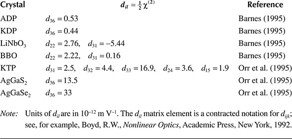
In Table 8.1, second-order nonlinear susceptibilities are listed for some well-known crystals.

Identities useful in this chapter are

k_{m} = \underline{n_{m} ω_{m}} (8.6)

$k_{m} = \underline{n_{m} ω_{m}} (8.6)$

k_{m} = \frac{2 π n_{m}}{λ_{m}} (8.7)

$k_{m} = \frac{2 π n_{m}}{λ_{m}} (8.7)$

and

n_{m} = (ε ω_{m})^{1 / 2} (8.8)

$n_{m} = (ε ω_{m})^{1 / 2} (8.8)$

TABLE 8.1
Second-Order Nonlinear Optical Susceptibilities

Images

8.2 Generation of Frequency Harmonics

In this section, a basic description of second harmonic, sum-frequency, and difference-frequency generation is given. The difference-frequency generation section is designed to describe some of the salient aspects of optical parametric oscillation.

8.2.1 Second Harmonic and Sum-Frequency Generation

Previously, Maxwell’s equations were applied to describe propagation in isotropic linear optical media. Here, the propagation of electromagnetic radiation in crystals is considered from a practical perspective consistent with the previous material on polarization.

Maxwell’s equations in the Gaussian system of units are given by (Born and Wolf 1999)

\nabla . B = 0 (8.9)

$\nabla . B = 0 (8.9)$

\nabla E = 4 π p (8.10)

$\nabla E = 4 π p (8.10)$

\nabla \times H = \frac{1}{c} (\frac{\partial D}{\partial t} + 4 π j) (8.11)

$\nabla \times H = \frac{1}{c} (\frac{\partial D}{\partial t} + 4 π j) (8.11)$

\nabla \times E = - \frac{1}{c} \frac{\partial B}{\partial t} (8.12)

$\nabla \times E = - \frac{1}{c} \frac{\partial B}{\partial t} (8.12)$

For a description of propagation in a crystal, we adopt the approach of Boyd (1992) and further consider a propagation medium characterized by ρ = 0, j = 0, and B = H. The nonlinearity of the medium introduces

D = E + 4 π P (8.13)

$D = E + 4 π P (8.13)$

As done in Chapter 5, taking the curl of both sides of Equation 8.12 and using Equation 8.13 lead to

\nabla \times \nabla \times E = - c^{- 2} (\nabla_{t}^{2} E + 4 π \nabla_{t}^{2} P) (8.14)

$\nabla \times \nabla \times E = - c^{- 2} (\nabla_{t}^{2} E + 4 π \nabla_{t}^{2} P) (8.14)$

which is the generalized wave equation for nonlinear optics. Here, $\nabla_{t}^{2} = (\partial^{2} / \partial t^{2})$ $\nabla_{t}^{2} = (\partial^{2} / \partial t^{2})$ .

Following Boyd (1992), it is useful to provide a number of definitions starting by separating the polarization into its linear and nonlinear components so that

P = P_{L} + P_{N L} (8.15)

$P = P_{L} + P_{N L} (8.15)$

followed by the separation of the displacement into

D = D_{L} + 4 π P_{N L} (8.16)

$D = D_{L} + 4 π P_{N L} (8.16)$

where:

D_{L} = E + 4 π P_{L} (8.17)

$D_{L} = E + 4 π P_{L} (8.17)$

Using this definition, the nonlinear wave equation can be rewritten as

\nabla \times \nabla \times E = - c^{- 2} (\nabla_{t}^{2} D_{L} + 4 π \nabla_{t}^{2} P_{N L}) (8.18)

$\nabla \times \nabla \times E = - c^{- 2} (\nabla_{t}^{2} D_{L} + 4 π \nabla_{t}^{2} P_{N L}) (8.18)$

In Chapter 5, for an isotropic material, we have seen that

D_{L} = ε E (8.19)

$D_{L} = ε E (8.19)$

For the case of a crystal, this definition can be modified to

D_{L} (r, t) = ε (ω) \cdot E (r, t) (8.20)

$D_{L} (r, t) = ε (ω) \cdot E (r, t) (8.20)$

which includes a real frequency-dependent dielectric tensor. Using Equation 8.20, the nonlinear wave equation can be restated as (Armstrong et al. 1962)

\nabla \times \nabla \times E (r, t) = - c^{- 2} [ε (ω) \cdot \nabla_{t}^{2} E (r, t) + 4 π \nabla_{t}^{2} P_{N L} (r, t)] (8.21)

$\nabla \times \nabla \times E (r, t) = - c^{- 2} [ε (ω) \cdot \nabla_{t}^{2} E (r, t) + 4 π \nabla_{t}^{2} P_{N L} (r, t)] (8.21)$

where:

E (r, t) = E (r) e^{- i ω t} + ... (8.22)

$E (r, t) = E (r) e^{- i ω t} + ... (8.22)$

and

P_{N L} (r, t) = P_{N L} (r) e^{- i ω t} + ... (8.23)

$P_{N L} (r, t) = P_{N L} (r) e^{- i ω t} + ... (8.23)$

Now, with the nonlinear wave equation established, we proceed to describe the process of second harmonic generation or frequency doubling. This is illustrated schematically in Figure 8.1 and consists in the basic process of radiation of ω₁ incident on a nonlinear crystal to yield collinear output radiation of frequency ω₂ = 2ω₁. We proceed as done in Chapter 5 using the identity

Images

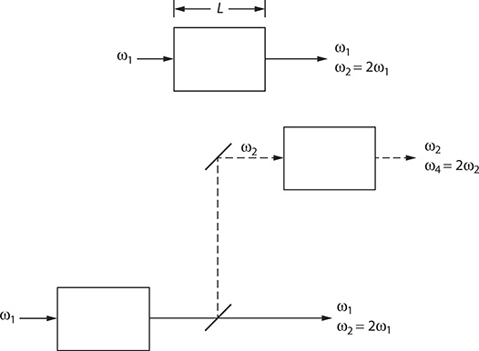
FIGURE 8.1 Optical configuration for frequency doubling generation.

\nabla \times \nabla \times E = \nabla \nabla E - \nabla^{2} E (8.24)

$\nabla \times \nabla \times E = \nabla \nabla E - \nabla^{2} E (8.24)$

The wave equation can be restated in scalar form as

\nabla^{2} E_{m} (z, t) = - c^{- 2} [ε (ω_{m}) \nabla_{t}^{2} E_{m} (z, t) + 4 π \nabla_{t}^{2} P_{m} (z, t)] (8.25)

$\nabla^{2} E_{m} (z, t) = - c^{- 2} [ε (ω_{m}) \nabla_{t}^{2} E_{m} (z, t) + 4 π \nabla_{t}^{2} P_{m} (z, t)] (8.25)$

After Boyd (1992), we use the following expressions for m = 2:

E_{m} (z, t) = A_{m} (z) e^{i k_{m^{Z}}} e^{- i ω_{m} t} + ... (8.26)

$E_{m} (z, t) = A_{m} (z) e^{i k_{m^{Z}}} e^{- i ω_{m} t} + ... (8.26)$

E (z, t) = E_{1} (z, t) + E_{2} (z, t) (8.27)

$E (z, t) = E_{1} (z, t) + E_{2} (z, t) (8.27)$

P_{m} (z, t) = P_{m} (z) e^{- i ω_{m} t} + ... (8.28)

$P_{m} (z, t) = P_{m} (z) e^{- i ω_{m} t} + ... (8.28)$

P_{1} (z) = 4 d A_{2} A_{1}^{*} e^{i (k_{2} - k_{1}) z} (8.29)

$P_{1} (z) = 4 d A_{2} A_{1}^{*} e^{i (k_{2} - k_{1}) z} (8.29)$

P_{2} (z) = 2 d A_{1}^{2} e^{i k_{1^{Z}}} (8.30)

$P_{2} (z) = 2 d A_{1}^{2} e^{i k_{1^{Z}}} (8.30)$

P (z, t) = P_{1} (z, t) + P_{2} (z, t) (8.31)

$P (z, t) = P_{1} (z, t) + P_{2} (z, t) (8.31)$

Following differentiation and substitution into the wave equation, the ∂²A₁/∂z₁ and ∂²A₂/∂z₂ terms are neglected so that the coupled amplitude equations can be expressed as (Boyd 1992)

\frac{d A_{1}}{d z} = i (\frac{8 π d ω_{1}^{2}}{k_{1} c^{2}}) A_{1}^{*} A_{2} e^{- i Δ k z} (8.32)

$\frac{d A_{1}}{d z} = i (\frac{8 π d ω_{1}^{2}}{k_{1} c^{2}}) A_{1}^{*} A_{2} e^{- i Δ k z} (8.32)$

and

\frac{d A_{2}}{d z} = i (\frac{4 π d ω_{2}^{2}}{k_{2} c^{2}}) A_{1}^{2} e^{i Δ k z} (8.33)

$\frac{d A_{2}}{d z} = i (\frac{4 π d ω_{2}^{2}}{k_{2} c^{2}}) A_{1}^{2} e^{i Δ k z} (8.33)$

where:

Δ k = 2 k_{1} - k_{2} (8.34)

$Δ k = 2 k_{1} - k_{2} (8.34)$

Integration of Equation 8.33 leads to

A_{2} A_{2}^{*} = (\frac{4 π d ω_{2}^{2}}{k c^{2}})^{2} A_{1}^{4} L^{2} [\frac{(\sin^{2} L Δ k / 2)}{(L Δ k / 2)^{2}}] (8.35)

$A_{2} A_{2}^{*} = (\frac{4 π d ω_{2}^{2}}{k c^{2}})^{2} A_{1}^{4} L^{2} [\frac{(\sin^{2} L Δ k / 2)}{(L Δ k / 2)^{2}}] (8.35)$

The above equation illustrates the nonlinear dependence of the frequency-doubled output on the input signal and indicates its relation to the (LΔk/2) parameter. This dependence implies that conversion efficiency decreases significantly as (LΔk/2) increases. The distance

Images

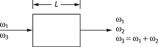
FIGURE 8.2 Optical configuration for sum-frequency generation.

L_{c} = \frac{2}{Δ k} (8.36)

$L_{c} = \frac{2}{Δ k} (8.36)$

is referred to as the coherence length of the crystal and provides a measure of the length of the crystal necessary for the efficient generation of second-harmonic radiation.

Sum-frequency generation is outlined in the third term of Equation 8.4 and involves the interaction of radiation at two different frequencies in a crystal to produce radiation at a third distinct frequency. This process is illustrated schematically in Figure 8.2 and consists in the normal incidence radiation of ω₁ and ω₂ onto a nonlinear crystal to yield collinear output radiation of frequency ω₃ = ω₁ + ω₂. Using the appropriate expressions for E_m(z, t) and P_m(z, t), in the wave equation, it can be shown that (Boyd 1992)

Δ k = k_{1} + k_{2} - k_{3} (8.37)

$Δ k = k_{1} + k_{2} - k_{3} (8.37)$

and the output intensity again depends on sinc²(LΔk/2).

The ideal condition of phase matching is achieved when

Δ k = 0 (8.38)

$Δ k = 0 (8.38)$

and it offers the most favorable circumstances for a high conversion efficiency. When this condition is not satisfied, there is a strong decrease in the efficiency of sum-frequency generation.

8.2.2 Difference-Frequency Generation and Optical Parametric Oscillation

The process of difference-frequency generation is outlined in the fourth term of Equation 8.4 and involves the interaction of radiation at two different frequencies in a crystal to produce radiation at a third distinct frequency. This process is illustrated schematically in Figure 8.3 and consists in the normal incidence radiation of ω₁ and ω₃ onto a nonlinear crystal to yield collinear output radiation of frequency ω₂ = ω₃ - ω₁.

Images

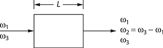
FIGURE 8.3 Optical configuration for difference-frequency generation.

Assuming that ω₃ is the frequency of a high-intensity pump laser beam, which remains undepleted during the excitation process, then A₃ can be considered a constant, and using an analogous approach to that adopted in Section 8.2.1, it is found that (Boyd 1992)

\frac{d A_{1}}{d z} = i (\frac{8 π d ω_{1}^{2}}{k_{1} c^{2}}) A_{3} A_{2}^{*} e^{i Δ k z} (8.39)

$\frac{d A_{1}}{d z} = i (\frac{8 π d ω_{1}^{2}}{k_{1} c^{2}}) A_{3} A_{2}^{*} e^{i Δ k z} (8.39)$

\frac{d A_{2}}{d z} = i (\frac{8 π d ω_{2}^{2}}{k_{2} c^{2}}) A_{3} A_{1}^{*} e^{i Δ k z} (8.40)

$\frac{d A_{2}}{d z} = i (\frac{8 π d ω_{2}^{2}}{k_{2} c^{2}}) A_{3} A_{1}^{*} e^{i Δ k z} (8.40)$

\frac{d A_{3}}{d z} = 0 (8.41)

$\frac{d A_{3}}{d z} = 0 (8.41)$

where:

Δ k = k_{3} - k_{2} - k_{1} (8.42)

$Δ k = k_{3} - k_{2} - k_{1} (8.42)$

If the nonlinear crystal involved in the process of frequency difference is deployed, and properly aligned at the propagation axis of an optical resonator, as illustrated in Figure 8.4, then the intracavity intensity can build to very high values. This is the essence of an optical parametric oscillator (OPO). Early papers on OPOs are those of Giordmaine and Miller (1965), Akhmanov et al. (1966), Byer et al. (1968), and Harris (1969). Recent reviews are given by Barnes (1995) and Orr et al. (2009).

In the OPO literature, ω₃ is known as the pump frequency, ω₁ as the idler frequency, and ω₂ as the signal frequency. Thus, Equation 8.42 can be restated as

Δ k = k_{P} - k_{S} - k_{I} (8.43)

$Δ k = k_{P} - k_{S} - k_{I} (8.43)$

Equations 8.39 and 8.40 can be used to provide equations for the signal under various conditions of interest. For example, for the case when the initial idler intensity is zero, and Δk ≈ 0, it can be shown that

A_{S} (L) A_{S}^{*} (L) \approx \frac{1}{4} A_{S} (0) A_{S}^{*} (0) (e^{γ L} + e^{- γ L})^{2} (8.44)

$A_{S} (L) A_{S}^{*} (L) \approx \frac{1}{4} A_{S} (0) A_{S}^{*} (0) (e^{γ L} + e^{- γ L})^{2} (8.44)$

where:

A_S(0) is the initial amplitude of the signal

Images

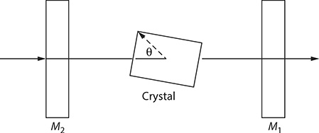
FIGURE 8.4 Basic OPO configuration.

Here, the parameter γ is defined as (Boyd 1992)

γ = (64 π^{2} d^{2} ω_{I}^{2} ω_{S}^{2} k_{I}^{- 1} k_{S}^{- 1} c^{- 4} | A_{P} |^{2})^{1 / 2} (8.45)

$γ = (64 π^{2} d^{2} ω_{I}^{2} ω_{S}^{2} k_{I}^{- 1} k_{S}^{- 1} c^{- 4} | A_{P} |^{2})^{1 / 2} (8.45)$

Equation 8.44 indicates that for the ideal condition of Δk ≈ 0, the signal experiences an exponential gain as long as the pump intensity is not depleted.

Frequency selectivity in pulsed OPOs has been studied in detail by Brosnan and Byer (1979) and Barnes (1995). Wavelength tuning by angular and thermal means is discussed by Barnes (1995). Considering the frequency difference

ω_{S} = ω_{P} - ω_{I} (8.46)

$ω_{S} = ω_{P} - ω_{I} (8.46)$

and Equation 8.43, it can be shown that for the case of Δk ≈ 0 (Orr et al. 1995)

λ_{s} \approx \frac{λ_{P} (n_{S} - n_{I})}{(n_{P} - n_{I})} (8.47)

$λ_{s} \approx \frac{λ_{P} (n_{S} - n_{I})}{(n_{P} - n_{I})} (8.47)$

which illustrates the dependence of the signal wavelength on the refractive indices. An effective avenue to change the refractive index is to vary the angle of the optical axis of the crystal, relative to the optical axis of the cavity, as indicated in Figure 8.4. For instance, Brosnan and Byer (1979) report that changing this angle from 45° to 49°, in a Nd:YAG laser-pumped LiNbO₃ OPO, tunes the wavelength from ~2 μm to beyond 4 μm. The angular dependence of refractive indices in uniaxial birefringent crystals is discussed by Born and Wolf (1999).

It should be mentioned that the principles discussed in Chapters 4 and 7 can be applied toward the tuning and linewidth narrowing in OPOs. However, there are some unique features of nonlinear crystals that should be considered in some detail. Central to this discussion is the issue of phase matching or allowable mismatch. It is clear that a resonance condition exists around Δk ≈ 0, and from Equation 8.44, it is seen that the output signal from an OPO can experience a large increase when this condition is satisfied. Thus, Δk ≈ 0 is a desirable feature. Here, it should be mentioned that some authors define slightly differently what is known as allowable mismatch. For instance, Barnes (1995) defines it as

Δ k = \frac{π}{L} (8.48)

$Δ k = \frac{π}{L} (8.48)$

which is slightly broader than the definition given in Equation 8.36.

The discussion on frequency selectivity in OPOs benefits significantly by expanding Δk in a Taylor series (Barnes and Corcoran 1976) so that

Δ k = Δ k_{0} + (\frac{\partial Δ k}{\partial x}) Δ x + \frac{1}{2!} (\frac{\partial^{2} Δ k}{\partial x^{2}}) Δ x^{2} + ... (8.49)

$Δ k = Δ k_{0} + (\frac{\partial Δ k}{\partial x}) Δ x + \frac{1}{2!} (\frac{\partial^{2} Δ k}{\partial x^{2}}) Δ x^{2} + ... (8.49)$

Here, this process is repeated for other variables of interest:

Δ k = Δ k_{0} + (\frac{\partial Δ k}{\partial θ}) Δ θ + \frac{1}{2!} (\frac{\partial^{2} Δ k}{\partial θ^{2}}) Δ θ^{2} + ... (8.50)

$Δ k = Δ k_{0} + (\frac{\partial Δ k}{\partial θ}) Δ θ + \frac{1}{2!} (\frac{\partial^{2} Δ k}{\partial θ^{2}}) Δ θ^{2} + ... (8.50)$

Δ k = Δ k_{0} + (\frac{\partial Δ k}{\partial λ}) Δ λ + \frac{1}{2!} (\frac{\partial^{2} Δ k}{\partial λ^{2}}) Δ λ^{2} + ... (8.51)

$Δ k = Δ k_{0} + (\frac{\partial Δ k}{\partial λ}) Δ λ + \frac{1}{2!} (\frac{\partial^{2} Δ k}{\partial λ^{2}}) Δ λ^{2} + ... (8.51)$

Δ k = Δ k_{0} + (\frac{\partial Δ k}{\partial T}) Δ T + \frac{1}{2!} (\frac{\partial^{2} Δ k}{\partial T^{2}}) Δ T^{2} + ... (8.52)

$Δ k = Δ k_{0} + (\frac{\partial Δ k}{\partial T}) Δ T + \frac{1}{2!} (\frac{\partial^{2} Δ k}{\partial T^{2}}) Δ T^{2} + ... (8.52)$

Equating the first two series, and ignoring the second derivatives, it is found that (Barnes 1995)

Δ λ = Δ θ (\frac{\partial Δ k}{\partial θ}) (\frac{\partial Δ k}{\partial λ})^{- 1} (8.53)

$Δ λ = Δ θ (\frac{\partial Δ k}{\partial θ}) (\frac{\partial Δ k}{\partial λ})^{- 1} (8.53)$

This linewidth equation shows a dependence on the beam divergence, which is determined by the geometrical characteristics of the pump beam and the geometry of the cavity. It should be noted that this equation provides an estimate of the intrinsic linewidth available from an OPO in the absence of intracavity dispersive optics or injection seeding from external sources. Barnes (1995) reports that for a AgGaSe₂ OPO pumped by an Er:YLF laser, the linewidth is Δλ = 0.0214 μm at λ = 3.82 μm.

Introduction of the intracavity dispersive techniques described in Chapter 7 produces much narrower emission linewidths. A dispersive OPO is illustrated in Figure 8.5. For this oscillator, the multiple-return-pass linewidth is determined by

Δ λ = Δ θ_{R} (R M \nabla_{λ} Θ_{G} + R \nabla_{λ} Φ_{P})^{- 1} (8.54)

$Δ λ = Δ θ_{R} (R M \nabla_{λ} Θ_{G} + R \nabla_{λ} Φ_{P})^{- 1} (8.54)$

where the various coefficients are defined in Chapter 7. It should be apparent that Equation 8.54 has its origin in

Images

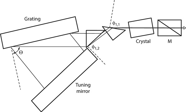
FIGURE 8.5 Dispersive OPO using a HMPGI grating configuration as described by Duarte. (Data from Duarte, F.J., Tunable Laser Optics, Elsevier Academic Press, New York, 2003.)

Δ λ = Δ θ (\frac{\partial θ}{\partial λ})^{- 1} (8.55)

$Δ λ = Δ θ (\frac{\partial θ}{\partial λ})^{- 1} (8.55)$

which is a simplified version of Equation 8.53. Hence, we have demonstrated a simple mathematical approach to arrive to the linewidth equation, which was previously derived using interferometric arguments in Chapter 2.

Using a dispersive cavity incorporating an intracavity etalon in a LiNbO₃ OPO excited by a Nd:YAG laser, Brosnan and Byer (1979) achieved a linewidth of Δν = 2.25 GHz. Also using a Nd:YAG-pumped LiNbO₃ OPO, and a similar interferometric technique, Milton et al. (1989) achieved single-longitudinal-mode emission at a linewidth of Δν ≈ 30 MHz.

A further aspect illustrated by the Taylor series expansion is that equating the second and third series, it is found that (Duarte 2003)

Δ θ = Δ T (\frac{\partial Δ k}{\partial T}) (\frac{\partial Δ k}{\partial θ})^{- 1} (8.56)

$Δ θ = Δ T (\frac{\partial Δ k}{\partial T}) (\frac{\partial Δ k}{\partial θ})^{- 1} (8.56)$

which indicates that the beam divergence is a function of temperature, which should be considered when contemplating thermal tuning techniques. Chapter 9 includes a section on the emission performance of various OPOs.

8.2.3 The Refractive Index as a Function of Intensity

Using a Taylor series to expand an expression for the refractive index yields

n = n_{0} + (\frac{\partial n}{\partial I}) I + \frac{1}{2!} (\frac{\partial^{2} n}{\partial I^{2}}) I^{2} + ... (8.57)

$n = n_{0} + (\frac{\partial n}{\partial I}) I + \frac{1}{2!} (\frac{\partial^{2} n}{\partial I^{2}}) I^{2} + ... (8.57)$

Neglecting the second-order and higher terms, this expression reduces to

n = n_{0} + (\frac{\partial n}{\partial I}) I (8.58)

$n = n_{0} + (\frac{\partial n}{\partial I}) I (8.58)$

where:

n₀ is the normal weak-field refractive index defined in Chapter 13 for various materials

The quantity (∂n/∂I) is not dimensionless and has units that are the inverse of the laser intensity or W^–1 cm². Using polarization arguments, this derivative can be expressed as (Boyd 1992)

\frac{\partial n}{\partial I} = \frac{12 π^{2} χ^{3}}{n_{0}^{2} (ω) c} (8.59)

$\frac{\partial n}{\partial I} = \frac{12 π^{2} χ^{3}}{n_{0}^{2} (ω) c} (8.59)$

This quantity is known as the second-order index of refraction and is traditionally referred to as n₂. Setting (∂n/∂I) = n₂, Equation 8.58 can be restated in its usual form as

Images

FIGURE 8.6 Simplified representation of self-focusing, due to n = n₀ + n₁I, in an optical medium due to propagation of a laser beam with a near-Gaussian intensity profile.

n (ω) = n_{0} (ω) + n_{2} (ω) I (ω) (8.60)

$n (ω) = n_{0} (ω) + n_{2} (ω) I (ω) (8.60)$

The change in refractive index, as a function of laser intensity, is known as the optical Kerr effect.

A well-known consequence of the optical Kerr effect is the phenomenon of self-focusing. This results from the propagation of a laser beam with a near-Gaussian spatial intensity profile since, according to Equation 8.60, the refractive index at the center of the beam is higher than the refractive index at the wings of the beam. This results in an intensity-dependent lensing effect as illustrated in Figure 8.6.

The phenomenon of self-focusing, or intensity-dependent lensing, is important in ultrafast lasers or femtosecond lasers (Diels 1990; Diels and Rudolph 2006), where it gives rise to what is known as Kerr lens mode locking (KLM). This is applied to spatially select the high-intensity mode-locked pulses from the background continuous-wave lasing. This can be simply accomplished by inserting an aperture near the gain medium to restrict lasing to the central, high-intensity, portion of the intracavity beam. This technique has become widely used in femtosecond laser cavities.

8.3 Optical Phase Conjugation

Optical phase conjugation is a technique that is applied to correct laser beam distortions, either intracavity or extracavity. A proof of the distortion correction properties of phase conjugation was provided by Yariv (1977) and is outlined here. Consider a propagating beam, in the +z direction, represented by

E (r, t) = A_{1} (r) e^{- i (ω t - k z)} + ... (8.61)

$E (r, t) = A_{1} (r) e^{- i (ω t - k z)} + ... (8.61)$

and the scalar version of the nonlinear wave equation given in Equation 8.25, assuming that the spatial variations of ε are much larger than the optical wavelength. Neglecting the polarization term, one can write

\frac{\partial^{2} A_{1}}{\partial z^{2}} + i 2 k (\frac{\partial A_{1}}{\partial z}) - (\frac{ε ω^{2}}{c^{2}} + k^{2}) A_{1} = 0 (8.62)

$\frac{\partial^{2} A_{1}}{\partial z^{2}} + i 2 k (\frac{\partial A_{1}}{\partial z}) - (\frac{ε ω^{2}}{c^{2}} + k^{2}) A_{1} = 0 (8.62)$

The complex conjugate of this equation is

\frac{\partial^{2} A_{1}^{*}}{\partial z^{2}} - i 2 k (\frac{\partial A_{1}^{*}}{\partial z}) - (\frac{ε ω^{2}}{c^{2}} + k^{2}) A_{1}^{*} = 0 (8.63)

$\frac{\partial^{2} A_{1}^{*}}{\partial z^{2}} - i 2 k (\frac{\partial A_{1}^{*}}{\partial z}) - (\frac{ε ω^{2}}{c^{2}} + k^{2}) A_{1}^{*} = 0 (8.63)$

which is the same wave equation of a wave propagating in the –z direction of the form:

E (r, t) = A_{2} (r) e^{- i (ω t + k z)} + ... (8.64)

$E (r, t) = A_{2} (r) e^{- i (ω t + k z)} + ... (8.64)$

provided

A_{2} (r) = a A_{1}^{*} (r) (8.65)

$A_{2} (r) = a A_{1}^{*} (r) (8.65)$

where:

a is a constant

Here, the presence of a distorting medium is represented by the real quantity ε (Yariv 1977). This exercise illustrates that a wave propagating in the reverse direction of A₁(r), and whose complex amplitude is everywhere the complex conjugate of A₁(r), satisfies the same wave equation satisfied by A₁(r). From a practical perspective, this implies that a phase-conjugate mirror (PCM) can generate a wave propagating in reverse, to the incident wave, whose amplitude is the complex conjugate of the incident wave. Thus, the wave fronts of the reverse wave coincide with those of the incident wave. This concept is illustrated in Figure 8.7.

A PCM, as depicted in Figure 8.8, is generated by a process called degenerate four-wave mixing (DFWM), which itself depends on χ⁽³⁾ (Yariv 1985). This process can be described considering plane wave equations of the form

Images

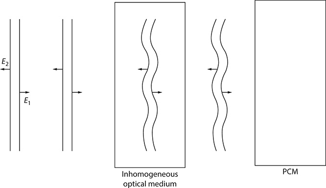
FIGURE 8.7 The concept of optical phase conjugation.

Images

FIGURE 8.8 Basic phase-conjugated laser cavity.

E_{m} (r, t) = A_{m} (r) e^{- i (ω t - k_{m} \cdot r)} + ... (8.66)

$E_{m} (r, t) = A_{m} (r) e^{- i (ω t - k_{m} \cdot r)} + ... (8.66)$

where:

m = 1, 2, 3, 4

k and r are vectors

Using these equations and the simplified equations for the four polarization terms (Boyd 1992),

P_{1} = 3 χ^{(3)} (E_{1}^{2} E_{1}^{*} + 2 E_{1} E_{2} E_{2}^{*}) (8.67a)

$P_{1} = 3 χ^{(3)} (E_{1}^{2} E_{1}^{*} + 2 E_{1} E_{2} E_{2}^{*}) (8.67a)$

P_{2} = 3 χ^{(3)} (E_{2}^{2} E_{2}^{*} + 2 E_{2} E_{1} E_{1}^{*}) (8.67b)

$P_{2} = 3 χ^{(3)} (E_{2}^{2} E_{2}^{*} + 2 E_{2} E_{1} E_{1}^{*}) (8.67b)$

P_{3} = 3 χ^{(3)} (2 E_{3} E_{1} E_{1}^{*} + 2 E_{3} E_{2} E_{2}^{*} + 2 E_{1} E_{2} E_{4}^{*}) (8.67c)

$P_{3} = 3 χ^{(3)} (2 E_{3} E_{1} E_{1}^{*} + 2 E_{3} E_{2} E_{2}^{*} + 2 E_{1} E_{2} E_{4}^{*}) (8.67c)$

P_{4} = 3 χ^{(3)} (2 E_{4} E_{1} E_{1}^{*} + 2 E_{4} E_{2} E_{2}^{*} + 2 E_{1} E_{2} E_{3}^{*}) (8.67d)

$P_{4} = 3 χ^{(3)} (2 E_{4} E_{1} E_{1}^{*} + 2 E_{4} E_{2} E_{2}^{*} + 2 E_{1} E_{2} E_{3}^{*}) (8.67d)$

into the generalized wave equation

\nabla^{2} E_{m} (z, t) = - c^{- 2} [ε (ω_{m}) \nabla_{t}^{2} E_{m} (z, t) + 4 π \nabla_{t}^{2} P_{m} (z, t)]

$\nabla^{2} E_{m} (z, t) = - c^{- 2} [ε (ω_{m}) \nabla_{t}^{2} E_{m} (z, t) + 4 π \nabla_{t}^{2} P_{m} (z, t)]$

eventually lead to expressions for the amplitudes, which show that the generated field is driven only by the complex conjugate of the input amplitude.

An issue of practical interest is the representation of a PCM in transfer matrix notation, as introduced in Chapter 6. This problem was solved by Auyeung et al. (1979), who, using the argument that the reflected field is the conjugate replica of the incident field, showed that the ABCD matrix (see Chapter 6) is given by

(\begin{matrix} A & B \\ C & D \end{matrix}) = (\begin{matrix} 1 & 0 \\ 0 & - 1 \end{matrix}) (8.68)

$(\begin{matrix} A & B \\ C & D \end{matrix}) = (\begin{matrix} 1 & 0 \\ 0 & - 1 \end{matrix}) (8.68)$

that should be compared to

(\begin{matrix} A & B \\ C & D \end{matrix}) = (\begin{matrix} 1 & 0 \\ 0 & 1 \end{matrix}) (8.69)

$(\begin{matrix} A & B \\ C & D \end{matrix}) = (\begin{matrix} 1 & 0 \\ 0 & 1 \end{matrix}) (8.69)$

for a conventional optical mirror. A well-known nonlinear material suitable as a PCM is CS₂ (Yariv 1985). Fluctuations in the phase-conjugated signal generated by DFWM in sodium were investigated by Kumar et al. (1984).

8.4 Raman Shifting

Stimulated Raman scattering (SRS) is an additional, and very useful, tool to extend the frequency range of fixed frequency and tunable lasers. SRS, also known as Raman shifting, can be accomplished by focusing a TEM₀₀ laser beam on to a nonlinear medium, such as H₂ (as illustrated in Figure 8.9), to generate emission at a series of wavelengths above and below the wavelength of the laser pump. The series of longer wavelength emissions are known as Stokes and are determined by (Hartig and Schmidt 1979)

v_{S_{m}} = v_{P} - m v_{R} (8.70)

$v_{S_{m}} = v_{P} - m v_{R} (8.70)$

where:

$v_{S_{m}}$ $v_{S_{m}}$ is the frequency of a given Stokes

ν_P is the frequency of the pump laser

ν_R is the intrinsic Raman frequency

m = 1, 2, 3, 4 ... for successively higher Stokes

For the series of shorter anti-Stokes wavelengths,

v_{A S_{m}} = v_{P} + m v_{R} (8.71)

$v_{A S_{m}} = v_{P} + m v_{R} (8.71)$

where:

$v_{A S_{m}}$ $v_{A S_{m}}$ is the frequency of a given anti-Stokes

It should be noted that $v_{S_{1}}$ $v_{S_{1}}$ and $v_{A S_{1}}$ $v_{A S_{1}}$ are generated by the pump radiation, while these fields, in turn, generate $v_{S_{2}}$ $v_{S_{2}}$ and $v_{A S_{2}}$ $v_{A S_{2}}$ . In other words, for m = 2, 3, 4 ..., $v_{S_{m}}$ $v_{S_{m}}$ and $v_{A S_{m}}$ $v_{A S_{m}}$ are generated by $v_{S_{(m - 1)}}$ $v_{S_{(m - 1)}}$ and $v_{A S_{(m - 1)}}$ $v_{A S_{(m - 1)}}$ , respectively. Hence, the most intense radiation occurs for m = 1 with successively weaker emission for m = 2, 3, 4... as depicted in Figure 8.10. For instance, efficiencies can decrease progressively from 37% (first Stokes), to 18% (second Stokes), to 3.5% (third Stokes) (Berik et al. 1985). For the H₂ molecule, ν_R ≈ 124.5637663 THz (or 4155 cm⁻¹) (Bloembergen 1967).

Using the wave equation and assuming solutions of the form

E_{S} (z, t) = A_{S} (z) e^{- i (ω_{S} t - k_{S} z)} + ... (8.72)

$E_{S} (z, t) = A_{S} (z) e^{- i (ω_{S} t - k_{S} z)} + ... (8.72)$

and

E_{P} (z, t) = A_{P} (z) e^{- i (ω_{P} t - k_{P} z)} + ... (8.73)

$E_{P} (z, t) = A_{P} (z) e^{- i (ω_{P} t - k_{P} z)} + ... (8.73)$

Images

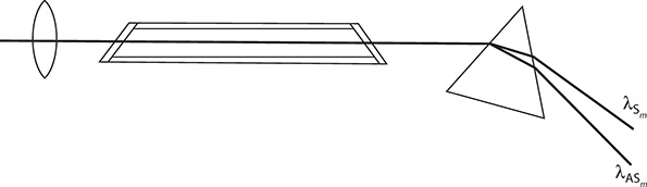
FIGURE 8.9 Optical configuration for H₂ Raman shifter. The output window and the dispersing prism are made of CaF₂.

Images

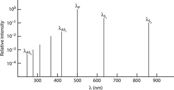
FIGURE 8.10 Stokes and anti-Stokes emission in H₂ for λ_P = 500 nm.

it can be shown, using the fact that the Stokes polarization depends on $χ^{(3)} E_{P} E_{P}^{*} E_{S},$ $χ^{(3)} E_{P} E_{P}^{*} E_{S},$ , that the gain at the Stokes frequency depends on the intensity of the pump radiation, the population density, and the inverse of the Raman linewidth, among other factors (Trutna and Byer 1980). It is interesting to note that the Raman gain can be independent of the linewidth of the pump laser (Trutna et al. 1979). A detailed description on the mechanics of SRS is provided by Boyd (1992).

SRS in H₂ has been widely used to extend the frequency range of tunable lasers, such as dye lasers. This technique was first demonstrated by Schmidt and Appt (1972) using room-temperature hydrogen at a pressure of 200 atm. This is mentioned since, albeit simple, the use of pressurized hydrogen requires the use of stainless steel cells and detailed attention to safety procedures. Using a dye laser with an emission wavelength centered around 563 nm, Wilke and Schmidt (1978) generated SRS radiation in H₂ from the eight anti-Stokes (at 198 nm) to the third Stokes (at 2064 nm) at an overall conversion efficiency of up to 50%. Using the second harmonic of the dye laser, the same authors generated from the fourth anti-Stokes to the fifth Stokes, as illustrated in Table 8.2, at an overall conversion efficiency of up to 75%. Using a similar dye laser configuration, Hartig and Schmidt (1979) employed a capillary waveguide H₂ cell to generate tunable first, second, and third Stokes spanning in the 0.7–7 μm wavelength range.

Using a dye laser system incorporating an MPL grating oscillator and two stages of amplification, Schomburg et al. (1983) achieved generation up to the thirteenth anti-Stokes at 138 nm. Brink and Proch (1982) reported on a 70% conversion efficiency at the seventh anti-Stokes by lowering the H₂ temperature to 78°K. Hanna et al. (1985) reported on a 90% conversion efficiency to the first Stokes using an oscillator-amplifier configuration for SRS in H₂.

In addition to H₂, numerous materials have been characterized as SRS media (Bloembergen 1967; Yariv 1975). Other gaseous media include I₂ (Fouche and Chang 1972), Cs (Wyatt and Cotter 1980), Ba (Manners 1983), Sn and Ti (White and Henderson 1983; Ludewigt et al. 1984), and Pb (Marshall and Piper 1990). A review on SRS in optical fibers is given by Toulouse (2005).

TABLE 8.2
Tunable Raman Shifting in Hydrogen

Anti-Stokes λ Range (nm)	Tunable Laser^a λ Range (nm)	Stokes λ Range (nm)^b
λ₄ ≈ 192 (δλ₄ ≈ 5.8)^c	275 ≤ λ ≤ 287	309 ≤ λ₁ ≤ 326
λ₃ ≈ 210 (δλ₃ ≈ 7.2)		355 ≤ λ₂ ≤ 378
λ₂ ≈ 229 (δλ₂ ≈ 8.9)		418 ≤ λ₃ ≤450
λ₁ ≈ 251 (δλ₁ ≈ 10.7)		505 ≤ λ₄ ≤ 550
		640 ≤ λ₅ ≤ 711

Source: Wilke, V., and Schmidt, W., Appl. Phys., 16, 151–154, 1978.

aSecond-harmonic from a dye laser.

bApproximate values.

cCorresponds to a quoted range of 188.7 nm ≤ λ₁ ≤ 194.5 nm. All other values are approximated.

8.5 Optical Clockwork

Perhaps the most well-known application of nonlinear optics in the laser optics field is in the generation of second, third, and fourth harmonics of some well-established laser sources, including the Nd:YAG laser. Table 8.3 lists the laser fundamental and its three harmonics. This frequency multiplication can be accomplished using nonlinear crystals such as KDP and ADP. Certainly, it should be apparent that the generation of frequency harmonics is not just limited to the Nd:YAG laser, but it is also practiced with a variety of laser sources including widely tunable lasers such as the Ti:Sappire laser and various fiber lasers (see Chapter 9).

One application that integrates various aspects of laser optics, including harmonic generation, is known as optical clockwork (Holzwarth et al. 2001). This involves the generation of a phase-locked white-light continuum for absolute frequency measurements. This is an idea originally outlined by Hänsch and colleagues in the mid- to late 1970s (Eckstein et al. 1978).

TABLE 8.3
Harmonics of the ⁴F_3/2 − ⁴I_11/2 Transition of the Nd:YAG Laser

Fundamental	Harmonics
ν ≈ 2.82 × 10¹⁴ Hz (λ ≈ 1064 nm)	2ν ≈ 5.64 × 10¹⁴ Hz (λ ≈ 532 nm)
	3ν ≈ 8.46 × 10¹⁴ Hz (λ ≈ 355 nm)
	4ν ≈ 1.13 × 10¹⁵ Hz (λ ≈ 266 nm)

The basic tools in this technique are a stabilized femtosecond laser, a nonlinear crystal fiber capable of self-modulation, a stabilized narrow-linewidth laser, and a frequency doubling crystal. Briefly, the concept consists in generating a periodic train of pulses, also known as a comb or ruler, with each pulse separated in the frequency domain by an interval Δ, for an entire optical octave. This is accomplished by focusing a high-intensity femtosecond laser beam onto a χ⁽³⁾ medium. This medium is a crystal fiber also known as a photonic crystal fiber whose refractive index behaves according to

n (t) = n_{0} + n_{2} I (t) (8.74)

$n (t) = n_{0} + n_{2} I (t) (8.74)$

Propagation in such medium causes red spread at the leading edge of the pulse and a blue spread at the trailing edge of the pulse since the field experiences a time-dependent shift described by (Bellini and Hänsch 2000)

Δ ω (t) = - \frac{ω_{0} n_{2} L}{c} [\frac{d I (t)}{d t}] (8.75)

$Δ ω (t) = - \frac{ω_{0} n_{2} L}{c} [\frac{d I (t)}{d t}] (8.75)$

Thus, a high intensity of ~20 fs pulse focused on a χ⁽³⁾ medium, a few centimeters long, can give rise to a continuum (Holzwarth et al. 2001).

The frequency-stabilized, and broadened, pulse train is made collinear with the fundamental of the narrow-linewidth stabilized laser, to be measured, and its second harmonic (Diddams et al. 2000). The combined laser beam containing the pulse train, ν, and 2ν, is then dispersed by a grating and two detectors are combined to determine the frequency beating between the pulse train with ν and 2ν, thus determining the beat frequencies δ₁ and δ₂. From Figure 8.11, the frequency difference (2ν − ν) is given by Diddams et al. (2000)

2 v - v = n Δ \pm (δ_{1} \pm δ_{2}) (8.76)

$2 v - v = n Δ \pm (δ_{1} \pm δ_{2}) (8.76)$

where:

Δ = \frac{v_{g}}{2 L} (8.77)

$Δ = \frac{v_{g}}{2 L} (8.77)$

Images

FIGURE 8.11 Schematics for determining the frequency difference (2ν − ν) in the optical clockwork approach. This is a simplified version of the intensity versus frequency diagram considered by Diddams et al. (Adapted from Diddams, S.A., et al., Phys. Rev. Lett., 84, 5102–5105, 2000.)

is determined by controlling L, which is the cavity length of the stabilized femtosecond laser (here, v_g is the group velocity). Using this method, Diddams et al. (2000) determined ν for an ¹²⁷I₂-stabilized Nd:YAG laser to be 281, 630, 111, and 740 kHz with an uncertainty of 50 Hz or 2 × 10⁻¹³. More recently, further refinement in optical clockworks has resulted in optical frequency synthesizers capable of providing an upper limit for the measurement uncertainty of several parts in 10⁻¹⁸ (Diddams 2010). Applications for optical combs include next-generation optical clocks and precision spectroscopy. In astronomy, applications include calibration sources for the search of exoplanets and measurement of fundamental constants of the early universe (Diddams 2010).

Problems

8.1 Use Maxwell’s equations to derive the generalized wave equation of nonlinear optics, that is, Equation 8.14.

8.2 Use Equations 8.39 and 8.40 to arrive at Equation 8.44 using the approximation Δk ≈ 0.

8.3 Use the scalar form of the wave equation (Equation 8.25) to arrive at Equation 8.62.

8.4 Derive the linewidth equation for an OPO, that is, Equation 8.53.

8.5 Determine the wavelengths for the Stokes radiation at m = 1, 2, 3 and for the anti-Stokes radiation at m = 1, 2, 3, 4, 5 for H₂, given that the laser excitation is at λ = 600 nm.

..................Content has been hidden....................

You can't read the all page of ebook, please click here login for view all page.

Table of Contents for
Chapter 8 Nonlinear Optics

8

Nonlinear Optics

8.1 Introduction

8.1.1 Introduction to Nonlinear Polarization

8.2 Generation of Frequency Harmonics

8.2.1 Second Harmonic and Sum-Frequency Generation

8.2.2 Difference-Frequency Generation and Optical Parametric Oscillation

8.2.3 The Refractive Index as a Function of Intensity

8.3 Optical Phase Conjugation

8.4 Raman Shifting

8.5 Optical Clockwork

Problems

Table of Contents for Chapter 8 Nonlinear Optics

Create new playlist

Sign In

Sign Up

Table of Contents for
Chapter 8 Nonlinear Optics