
which, written in polar coordinates, that is yields

and reduces to

because of the rotation-invariance of g, that is  In view of the definition of em,n,r in (2.5) this yields

which shows that the orthogonality relationship with respect to m is preserved, thatis  if m ≠ m′. Let
  and
and

then one may express the full scalar product as follows

Again, one can define a mutual angle detection algorithm, which approximatesthe best-matching rotation angle θ and in the course of the computation calculatesthe

When choosing a finite-dimensional frequency set Φr,ε, again the values of the function at the boundary, when expanded in the corresponding subspace, will lack a certain accuracy. When using a suitable intra-patchweight g, for instance a Gaussian weight (see (2.1)) with sufficiently small standard deviation parameter σ, to the values close to the boundary it will not be given a significant weight and the computations presented above will be almost error-free for the comparison of sampled signals.
Summarizing, we have developed a new way of computing the introduced error functions of the patch non-local means (2.2) and the patch non-local Poisson (2.3) for the best rotation angle θ, based on computations of suitable scalar products between the two patches. In Section 4.3, we will present how to practically implement the derived methods for application in exemplar-based inpainting algorithms.
4.3Rotation invariant exemplar-based inpainting
In Section 4.1, the underlying ideas of exemplar-based image inpainting were outlined. Now we want to introduce suitable energy functionals, whose alternating minimization schemes coincide with the exemplar-based image inpainting algorithm. The focus of this section is to discuss practical issues related to the implementation of such an algorithm, using the tools which we developed in the previous section. We will work with the so-called patch non-local means error function (2.2) and the gradient-based patch non-local Poisson error function (2.3). Further properties of the functionals, such as the existence of minimizers and convergence results of the alternating minimization algorithm to critical points, will be analyzed thoroughly in Section 4.4.
In addition to the choice of the intra-patch error function here again denoted generically with ϵ, we will add a selectivity parameter T ≥ 0 acting as a multiplier of a suitable regularizer. The case T > 0, as we will work out later, has a denoising effect. In fact, a similar method to the variational image inpainting has also been used for image denoising, cf. [9, 39, 41]. For inpainting problems on images which are (almost) free of noise we will give reasons why the case T = 0 is more suitable.
Let us discuss the influence of the selectivity parameter T. When we are looking for matching patches to a given patch px, where the available patches (py,θ)y,θ are given by all possible midpoints y ∈ Õ c and all possible rotations of angle θ ∈ [0, 2π], we are measuring the similarity between the two patches with a suitable distance function by computing ϵ(px − py,θ). The smaller the according error is, the closer the information of a patch py,θ is to px and also the more we can rely on it for the inpainting task. A selectivity parameter T > 0 will imply the use not only of the best-matching patch to update the image, but also the use of the information of multiple patches. Their contribution shall be weighted correspondingly to the degree of match. In the limit for T → ∞we will be less “picky” and have a uniform weight on all possible patches (py,θ)y,θ independent of their actual similarity to px. The more interesting case is for T close to zero, where we give a strong emphasis on the similar patches and have almost no weight on the others. As T = 0, we will only pick one patch, the patch that is minimizing ϵ(px − py,θ). From the analytic point of view, the object describing the weight function of contributions of the patches (py,θ)y,θ for px is a probability measure νx(y, θ). A visualization of the influence of the selectivity parameter is given in Figure 7.
For T > 0 this probability distribution is absolutely continuous with respect to the Lebesgue measure and thus can be rewritten in form of a density function w(x, y, θ), where x ∈ Õ are the points in the (extended) inpainting domain. Because of the factthat, for a fixed x, νx is a probability measure, we have that  for almost every x in Õ .
When T = 0, the probability measures νx are Dirac measures giving full weight to the best-matching patch, they do not have a density function as they are not absolutelycontinuous with respect to the Lebesgue measure. We will take a closer look at this case in Section 4.4.

4.3.1Patch non-local means
We will now discuss the case of an L2-norm based error function with an intra-patch weight function g, where

The weight function g is assumed to be in  and radially symmetric, that is g(h) = g(|h|). Without loss of generality we will also assume that ∫ℝ2 g(h)dh = 1.
4.3.1.1Selectivity parameter T = 0
In the case T = 0 we will consider the following functional

under the restriction that the push-forward measure (in the sense of [2, Def. 1.70]) π#ν = ℒ2|Õ , where π : Õ × Õ c × [0, 2π] → O ̃ is the projection on the first component. This restriction guarantees that the extracted (or disintegrated) measures νx are probability measures. (See Section 4.4.1.3 for details.)
Let us now discuss why the alternating minimization scheme on E0(u, ν) coincides with the image inpainting algorithm loosely described in Section 1. By an alternating minimization scheme we mean the iterative process of fixing u and updating ν as the minimizer of E0(u, ⋅), then updating the image information u as a minimizer of E0(⋅, ν) with ν fixed. We will also understand the influence of the intra-patch weight function g.
If u is fixed and we minimize (3.1) with respect to ν, then for every x ∈ Õ we are searching for the probability measure νx(y, θ) such that

is minimal, since we can assume  for any (y, θ). Assuming that there is a unique minimizer (y∗, θ∗) of the distance function, the minimal probability measure would be νx(y, θ) = δ(y∗,θ∗)(y, θ), the Dirac measure in (y∗, θ∗). If thereis more than one minimizer, say a family of minimizers
  any convex combi- nation of the Dirac measures
  would minimize (3.2). As will be addressed in Lemma 4.4
  is uniformly Lipschitz with respect to x, y, and θ and we may assume that for each x a minimizer (y∗, θ∗) exists, whenever (y, θ) can be chosen from the closed set cl(Õ c) × [0, 2π]. Choosing for every x the corresponding νx and combining them into a Radon measure ν, such that π#ν = ℒ2|Õ , we obtain the minimizer ν(u) of E0(u, ⋅). Notice that for the application to discrete digital images the described process is equivalent to the calculation of a one-to-one correspondence x ↦ (y(x), θ(x)),where for all x the pair (y(x), θ(x)) is such that
  is minimal.
In the image update step ν is fixed and we minimize E 0(⋅, ν) with respect to u. The information obtained from the patches Rθ(x)pû (y(x)) is merged to form a new iterate of the inpainted image. Here the intra-patchweight function g plays a significant role. We compute the Euler–Lagrange equation

and, by appropriate use of test functions, deduce that

Because of the radial symmetry of g, the fact that ∫ℝ2 g(h)dh = 1 and the fact that νxis a probability density for all x ∈ O we have that

and conclude from (3.3) that

Let us discuss the above equation in the continuous setting. Because of the fact that the patches around nearby points x, x′, look very similar, it is often the case, that the best-matching patches, not only also look similar, but also are centered in nearby points y, y′, having the same displacement as x and x′. As a consequence inpainting images constructed by exemplar-based inpainting algorithms, by use of (3.4), have regions inside the inpainting domain,which are rigidly copied from a region outside the inpainting domain. In a point within such a region, which is not close to a boundary to another region, the local energy value of (3.1) in x, that is  is zero and hence optimal. Figure 8 depicts the case of copy regions and transition bands. The minimization of the energy in (3.1) promotes the construction of large copy regions with transitions that in the best case match perfectly, if not so, are at least almost matching. The theory of copy regions extends without error to the discrete case of exemplar-based inpainting without rotations, since then grid points are always congruent. Because of the rotations this congruence does not hold for discrete rotation invariant exemplar-based inpainting algorithms and therefore within copy regions one still produces a (relatively) small error. However, as our numerical results show, in practice this does not have significant negative effects on the quality of the inpainting results.

4.3.1.2Selectivity parameter T > 0
For T > 0, the “fuzzy” correspondence case, we consider the following functional

subject to

where, for each x, w(x, ⋅, ⋅) are probability densities which regulate the influence of the known patches py,θ.
We shall now examine the Euler–Lagrange equation to get an insight into how w is chosen in the course of the alternating minimization scheme. For a fixed u and minimizing with respect to w, we obtain

which is solved by

where

is the normalization to make w a probability density (to fulfill (3.6)).
We note that w(x, y, θ) is large whenever  relatively small and vice versa. If we let T → ∞we obtain w(x, y, θ) ≡ const, the uniform distribution. Conversely, for T → 0 the probability density of each point x, w(x, ⋅, ⋅), concentrates around the points (y(x), θ(x)), where ‖pu(x) − Rθ(x)pû (y(x))‖g is minimal. Intuitively, one can already see a link between E0 and ET, T > 0. We will further analyze this relationship and present a related result in Proposition 4.8.
For a fixed w and minimizing with respect to u one can proceed as above, where T = 0, to obtain an equation like (3.4), which here reads as

In contrast to the case of copy regions and transition bands in Figure 8 (where T = 0), here we have a smoothing effect for every pixel. This reduces, if present, noise on the image data but at the same time reduces details in the inpainting image.
4.3.1.3Correspondence update step
We shall now discuss how the correspondence update step for ET, T ≥ 0, can be implemented and discuss issues which occur in this context.
4.3.1.3.1 T = 0
As discussed above, the task is to compute a one-to-one correspondence
where for all x the correspondence maps onto φ(x) = (y(x), θ(x)) is such that ‖pu(x) − is minimal among all possible choices of (y, θ) ∈ cl(Õ c) × [0, 2π].
Obviously, this problem is highly non-convex and hence the detection of (y(x), θ(x)) is quite expensive. On the basis of the theory from the previous section we proposethe following procedure:
Algorithm 3.1 (Correspondence update step for E0). Input: A suitable frequency set
Φr,ε, representing a set of em,n,r where m ≥ 0.
For x ∈ Õ :
- Extract px = pu(x),
- For m in Φr,ε compute

- For y ∈ Õ c:
(a)For m in Φr,ε compute ⟨gpu(x)(m) , pû (y)⟩ℓ2 ,
(b)Calculate rotation angle θ(y) = arg(Mg(pu(x), p̂u(y))),
(c)Compute  by CH-moment scalar product, that is

4.Set φ(x) = (y∗(x), θ(y∗(x))), where y∗ is minimizing
We shall give some comments on the implementation of Algorithm 3.1. Let us first recall the importance of choosing a suitable frequency set Φr,ε containing pairs (m, n) such that the corresponding Circular Harmonics  form a basis for a sufficiently large subspace. Since images are real signals, we have seen that it is sufficient to consider em,n,r’s, m ≥ 0, because they preserve all information. Also for nearly bandlimited functions and a certain sampling grid it is suitable to only choose em,n,r’s which have a relatively small predominant frequency (see Figures 4, 6 and details in Section 4.2.2.1). The em,n,r’s, m = 0, are not needed for the rotation angle detection, however, we do need them for the calculation of the scalar product in step 3(c).
For computation of  it is necessary that the extracted patch is a disk of oddinteger diameter along the grid axes; only then does the midpoint of the patch coincide with x. Then for each (m, n) ∈ Φr,ε we compute the CH-moment with the usualcomplex ℓ2-scalar product on
  Then for all m inΦr,ε the complex vector
  (on Br(0) ∩ ℤ2) is computed as sum over the complexvectors em,n,r multiplied by the computed CH-moments
Let us now propose an efficient calculation for step 3 which is based on matrix computations. Let U ̂ be a rectangular matrix, of dimensions h × w with image data obtained from Oc (see Figure 9). Then from each position (i, j) in the matrix Û , which has a distance of at least r to the boundary of the matrix, the patch pû (i, j) is contained in Û . Let us denote the set containing these (i, j)’s by ? = {(i, j) ∈ ℤ2 |r ≤ i < h −r and r ≤ j < w − r}. The idea is to compute  atonce. Therefore, we consider a complex-valued matrix
  of the samedimensions as Û , that is h × w, which consists of zeros except for the entries which represent
 These are translated modulo h × w such that the center of the disk coincides with theleft upper corner of
  that is (i, j) = (0, 0), see also explanatory Figure 9.

 are translatedsuch that the origin coincides with the entry at (0, 0) (here this is shown for px instead of

Finally, let  k modulo h × w. Then theconvolution of the two matrices
  and U is such that
for all (i, j) ∈ ?. For the (i, j)’s which are not in ? the patch is not contained in U and is considered to be continued by repetition. In practice, when covering Õ c with multiple matrices (Û i)i they should be chosen with an overlap of r pixels, such that any patch pû (y) whose support is completely contained in Õ c is considered. Then, by applying the convolution theorem [3], we have that

and hence ⟨gpu(x)(m) , pû (i, j)⟩ℓ2 , (i, j) ∈ ?, can efficiently be calculated by three fast Fourier transforms (FFT) (two forward and one inverse), here denoted by ℱ.
The calculation in step 3(a) is executed separately for every m and the overall computation time essentially depends on the time required for the convolution. Hence the computation time of the Algorithm 3.1 can be optimized by leaving out larger m’s, which include just few em,n,r’s. Instead of using a frequency set like the one in Figure 6, one might also use a frequency set as is shown in Figure 10 for an approximative and fast computation. The approximation is the more accurate, the lower the respective angular frequencies of the patch are, since these are represented by em,n,r’s whose m is small.
Once the computations of step 3(a) are complete, one can run the mutual angle detection algorithm to compute Mg (see (2.31)), where the circular sum operations are acting component-wise. The argument of the complex number at entry (i, j) ∈ ? then is the detected rotation angle θ(i, j).
For step 3(c), we recall that  due to (2.27) can be rewritten as

Since the datum u ̂ is not changed during the iterative algorithm, the  y ∈ Õ c, can be precalculated once in the initialization phase of the inpainting algorithm. However,
  needs to be computed anew at every iteration, since of course u is being changed in course of the inpainting process. As was discussed in (2.30), the computation of ⟨pu(x), Rθpû (y)⟩g can be done using the computed
  (3.11). We have that

Finally, in step 4, one needs to pick the pair (y, θ(y)) which minimizes

Note that due to the fact that we only choose one angle θ(y) at a time makes it possible to have rotation angles which are as accurate as the machine precision. We will see that this can not be realized in the case where T > 0.
Given one patch px of diameter 27 pixels and a frequency set of Circular Harmonics depicted in Figure 10, a laptop computer with 4 CPU kernels (Intel® Core™ i7 CPU M 620@ 2.67GHz) and 4 GB RAM needs about a second to compute the best-matchingpatch py,θ from a matrix U ̂ of dimensions ∼ 1000 × 500. This is about 4 times longer than an optimized computation of  for each py from U ̂ without rotations. Hence, with the proposed algorithm one can cover a much broader variety of patches (any rotation angle is possible) than in a method, where only the four rotations of 0∘, 90∘, 180∘, and 270∘ are considered (these can easily be calculated since the image grid points are given on a perpendicular lattice), in roughly the same amount of time!
By this we stress very much the efficiency of the proposed method, in particular because in [41, Section 3.2, Figure 9] the authors found that 90∘-rotations are too coarse to give a significant improvement. In contrary, allowing for arbitrary rotation angles provides a much better image recovery, as we shall demonstrate in our numerical results in Section 4.3.3. [41] also mention obtaining better results for more finely sampled sets of rotation angles, however, they claim that they were not yet practically viable due to the significant increase in computational cost. With the present method we show that we can definitively overcome such limitations.
The algorithm can be easily parallelized. Since the algorithm runs a loop over x ∈ Õ and the loop is closed, in the sense that each process is independent of the others, they can be executed in parallel. The algorithm we propose was eventually implemented in a client/ server architecture. While the client is performing the inpainting algorithm and sends patches px to the server, the server is performing the search for the best-matching patch and sends back the information (y(x), θ(x)) to the client. Thus, the program could easily be extended to the case of multiple servers, each performing the search for the best-matching patch for different patches. The computation time for Algorithm 3.1 then reduces by a factor of about (Ncomp)−1, where Ncomp denotes the number of available computers running the server program.
4.3.1.3.2 T > 0
In the case of a fuzzy correspondence w(x, y, θ) every patch py,θ is given a weight corresponding to the degree it matches to px measured in the respective error function. For numerical treatment the number of possible rotation angles thus needs to be discretized. Let us therefore consider a finite family of rotation angles θk, k = 1, . . . , N rot and the following algorithm:
Algorithm 3.2 (Correspondence update step for ET, T >0). Input: A suitable frequency
set Φr,ε, representing a set of em,n,r where m ≥ 0.
For x ∈ Õ :
1.Extract px = pu(x),
2.For m in Φr,ε compute
3.For y ∈ Õ c:
(a)For m in Φr,ε compute ⟨gpu(x)(m) , pu(y)⟩ℓ2 ,
(b)For k = 1, . . . , Nrot compute  with scalar product computed from
4.For x ∈ O, y ∈ Oc and θ = θk, k = 1, . . . , Nrot,set w(x, y, θ) to be  where Z(x) is a normalization constant to makew(x, ⋅, ⋅) a probability density.
Practically, up to step 3(a), one proceeds as in Algorithm 3.1 and computes  (i, j)’slike in (3.11). Then for the computation of
  the scalar product for the angle dependent term is calculated by:

We note that for a given patch radius r, to achieve an accuracy which is comparable to the resolution of the sampling lattice of the image, a suitable choice of the number of rotations N rot is ∼ 2πr. Still, the computation of w(x, y, θ) in Algorithm 3.2can be done comparably fast: Exploiting the self-steerability property of the CircularHarmonics (2.6), once the complex matrices  are computed, the computationof
  can be accomplished faster than an explicit computation of these terms based on an angle-by-angle computation.
4.3.1.4Image update step
In the image update step, the inpainting image u is updated according to the correspondence which has been calculated in the image update step. Again, it makes senseto look separately at the cases T = 0 and T > 0.
4.3.1.4.1 T = 0
We have found in (3.4) that the updated u can be computed by

where νx(y, θ) = δ(y∗,θ∗)(y, θ) is the Dirac measure in the point (y∗, θ∗) such that the patch Rθ∗pû (y∗) is closest to pu(x) in the error norm ‖⋅ ‖g. The equation can be reformulated, using the fact that dνx is a Dirac measure for x ∈ Õ , to obtain

In the discrete case, since each x ∈ Õ has only one patch which gives contributions to u, #Õ patches need to be considered. The best-matching patch to px, py(x),θ(x), contributes to a pixel z near x, if |z − x| ≤ r. When updating u(z), the weight given to the information from this patch is g(|z − x|).
In the discrete setting, when the image data is only given on a two-dimensional grid (which can be identified with a subset of ℤ2), we do not possess the image data of a patch which is rotated by an arbitrary angle θ. Therefore, one needs to be able to compute the values which lie on the grid after rotation. This can be done with certain (spline) interpolation rules or, as was done in our implementation, also be accomplished by use of the Circular Harmonics basis. Let us briefly depict how this can be done and show some examples of rotated patches.
Given some patch py and a rotation angle θ, we proceed as follows. The moments of the patch function for m > 0 and (m, n) ∈ Φε,r are calculated. The real part of the moments is multiplied by 2 and subtracted from the patch. The moments are multiplied by eimθ and, again under consideration of the factor 2, added to the patch. Since we are working with real signals we can reason as in (2.10) to justify the described procedure.
4.3.1.4.2 T > 0
As stated in (3.9) we need to compute

In general one proceeds as in the case T = 0. However, in contrast to νx, the probability measures w(x, ⋅, ⋅) are no Dirac measures and hence we have to consider a lot more patches. Actually, we have that w(x, y, θ) > 0 for any choice of (x, y, θ), whenever w is chosen as in the Euler–Lagrange equation (3.7). Hence the number of patches which contribute to the inpainting image now is N rot ⋅ #Õ c, where N rot, the number of rotations, is ∼ 2πr. This results in a significantly higher computational effort. As statedbefore, in comparison to the case T = 0 one has more of a smoothing effect reducing noise but also the quality of the details in the inpainting image. Consequently, the case T = 0 is more relevant for inpainting problems, especially when the image data in Õ c, represented by û, can be considered to be (almost) free of noise.
4.3.2Patch non-local Poisson
4.3.2.1Selectivity parameter T = 0
In the case T = 0 we consider the following functional

under the restriction that π#ν = ℒ2|Õ , where π : Õ × Õ c × [0, 2π] → Õ is the projection on the first component. This restriction guarantees that the extracted (or disintegrated) measures νx are probability measures (see Section 4.4.1.3 for details).
We proceed as in Section 4.3.1.1 to show that for fixed u a minimizing ν is given, when for every x ∈ Õ the probability measure νx(y, θ) is such that

is minimal, since  for any (y, θ). Assuming that there is a unique minimizer (y∗, θ∗) the chosen probability measure νx(y, θ) would be νx(y, θ) = δ(y∗,θ∗)(y, θ) the Dirac measure in (y∗, θ∗). If there is more than one minimizer, say a family of minimizers
  any convex combination of theDirac measures
  would minimize (3.2∗). ∗As will be addressed in Lemma 4.15
 is uniformly Lipschitz with respect to x, y, and θ and we may hence assume that for each x a minimizer (y∗, θ∗) exists, whenever (y, θ) can be chosen from the closed set cl(Õ c) × [0, 2π]. Choosing for every x the corresponding νx and combining them to a Radon measure ν such that π#ν = ℒ2|Õ we obtain the minimizer ν(u) of E∇,0(u, ⋅). Notice that for the application to discrete digital images the described process is equivalent to the calculation of a one-to-one correspondence x ↦ (y(x), θ(x)), where for all x the pair (y(x), θ(x)) is such that
 is minimal.
We now compute the Euler–Lagrange equation for u:

∀φ ∈ W1,2(O), and proceed as in Section 4.3.1.1 and obtain that u solves the Euler– Lagrange equation, if it is the (weak) solution of the Poisson equation

where

Consequently, in the image update step of the patch non-local Poisson model, a partial differential equation of the form (3.18) needs to be solved.
4.3.2.2Selectivity parameter T > 0
For T > 0, the fuzzy correspondence case, we consider the following functional

subject to

where w(x, ⋅, ⋅) are probability densities for each x which regulate the influence of the known patches py,θ.
Analogously to Section 4.3.1.2, we have that the solution of the Euler–Lagrange equation of E∇,T(u, ⋅) for fixed u is given by

where

is the normalization to make w a probability density (to fulfill (3.21)).
For a fixed w and minimizing with respect to u one can proceed as above, where T = 0, to obtain a Poisson equation similar to (3.18):

where

4.3.2.3Correspondence update step
The correspondence update step is for both T = 0 and T > 0 quite similar to the patch non-local means model. Therefore, one basically proceeds as in Algorithms 3.1 and 3.2. The only difference is that we need to compute terms of the form

and hence one needs to calculate the following quantities

The quantities  do not change during the iterations of the inpainting algorithm and are precomputed at the beginning.
We recall the definition of p̃x,g from Section 4.2.5.2 (see (2.44)):

where

and

Note that, when ∂g(ρ)/∂ρ can be computed analytically (for instance when g is chosena Gaussian, see (2.1)), then the functions  can be evaluated analytically in anypoint (ρ, θ) ∈ ℝ2 since

and thus the evaluation of the formula in (3.28) requires not much more computational effort than for terms of the form  (see (3.27) and definition of the CircularHarmonics (2.5)). Furthermore, as was shown in Section 4.2.5.2, we have that

and in particular, for px = pu(x),

Using this formula, also the norms  can be computed. Then the gradient is evaluated analytically and no finite difference approximations are needed.
Choosing a suitable frequency set Φr,ε, we have the following algorithm.
Algorithm 3.3 (Correspondence update step for E∇,0). Input: A suitable frequency set
Φr,ε, representing a set of em,n,r where m ≥ 0.
For x ∈ Õ :
1.Extract px = pu(x),
2.For m in Φr,ε compute
3.For y ∈ Õ c:
(a)For m in Φr,ε compute
(b)Calculate rotation angle θ(y) = arg(Mg,∇(pu(x), pû (y))),
(c)Compute  by CH-moment scalar product, that is
4.Set φ(x) = (y∗(x), θ(y∗(x))), y∗ minimizer of
The computations of the scalar products in step 3(a) can again be executed by an FFT-based convolution, see (3.10).With similar modifications to Algorithm 3.2 one obtains an algorithm for the correspondence update step for E∇,T, T > 0.
The statements on computation time and parallelization for the correspondence update steps of ET, T ≥ 0, extend without change to the cases E∇,T, T ≥ 0, which we have been discussing in this section.
4.3.2.4Image update step
As we have seen in Section 4.3.2.1, the image update step of the alternating minimization scheme of E∇,0 requires the solution of a partial differential equation of the form

where
We shall firstly discuss how to compute the right-hand side div υ(ν)(x), x ∈ O, efficiently and thereafter how to implement solving of the partial differential equation.
We observe that, using the fact that dνx is a Dirac measure for any x ∈ Õ , for x ∈ O we have that

Comparing (3.33) to (3.15), we see that the right-hand side of (3.31) can be computed in a similar way to the image update step of E0 and the only difference is given by the fact that we do not consider Rθ∗(x)pû (y∗(x)), but Rθ∗(x)Δpû (y∗(x)). The values of the contributing patches can easily be calculated using the Circular Harmonics expansion, since the em,n,r’s are eigenfunctions of the Laplacian (see (2.34), (2.35), and Section 4.2.5.1).
For a numerical treatment of (3.31) one can use a standard finite element method (FEM) solver routine, for instance FreeFEM. For the image update only these function values of u are needed which are part of the image grid. Hence, for an efficient computation, the partial differential equation should be solved on a regular grid which coincideswith the image grid (for rectangular inpainting domains of dimensions h ×w this can be achieved by using the FreeFEM command mesh Th=square(h+2,w+2);, cf. [36]).
Notice that in the case T > 0, again, the number of patches which need to be considered is significantly larger and, consequently, the case T = 0 is more relevant for inpainting problems, especially when the image data in Õ c, represented by û, can be considered to be (almost) free of noise.
4.3.2.5Complexity and parallelization
The method described above is FFT based in the patch search and it has complexity ?(r2Mlog(M)), where r > 0 is the radius of the circular patch and M is the number of pixels in the searched image, see [32], p. 2081, for the detailed computation of the complexity. This is precisely the same complexity as the PatchMatch algorithm by [11, 12] without implementation of any rotation invariance! The library we implemented is fully parallelizable on clusters of computers, since the program is based on a client/ server architecture. The client sends individual patches to an available server for the patch to be compared to all possible patches in an image, considering arbitrary mutual rotations. A cluster of listening servers thus allows the parallel treatment of multiple patches and the comparisons, both L2-based and gradient-based, can potentially be executed very fast, depending on the number of available computers running the server program in the cluster. An additional level of parallelization can be achieved by splitting further the computation according to levels m of the circular harmonic spaces Φr,ε.
4.3.3Numerical experiments
We shall now go through a number of numerical results of the rotation invariant exemplar-based inpainting algorithm using the patch non-local means scheme, that is, the algorithm whose practical implementation was discussed in Section 4.3.1.
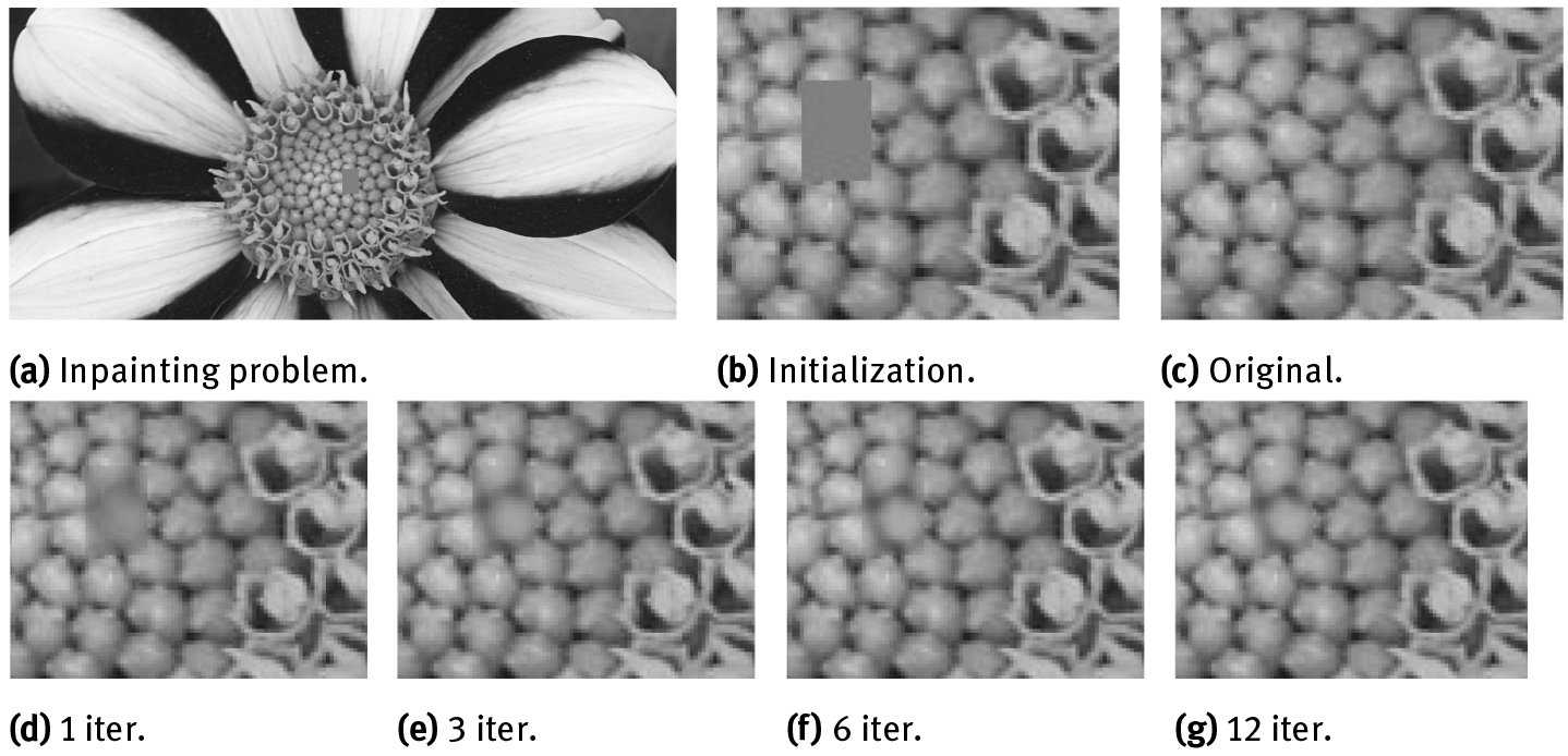
Before we go into the details of the influence of the parameters and the ability of recovering both geometry and structure, let us first show an example, where the presented exemplar-based inpainting algorithm yields impressive results in the recovery of repetitive textures. To this purpose, we consider the inpainting problem in Figure 11, depicting an application of the rotation invariant patch non-local means scheme. Even though the initialization value does not contain any useful information, the algorithm just needs a few iterations for a successful recovery of the structure in the center part of the flower. It is well known that exemplar-based inpainting algorithms perform well on textures, indeed they are also called texture-oriented inpainting methods (Section 4.1.1.2).
Let us now examine the ability of such algorithms to recover geometry and structures, in dependence of the parameters, the initialization, the number of iterations, and, of course, the benefit of adding rotation invariance as an additional degree of freedom.
4.3.3.1Dependence on choice of parameters
Once the inpainting problem is defined, that is the function û is defined in Oc and the initialization u0 inside the inpainting domain O is defined, the only parameters which we are free to choose are the patch diameter d and the intra-patchweight function g. As announced earlier, we will be using a Gaussian probability density function with zero mean and isotropic standard deviation σ. Then the choice of σ completely determines g. We shall now examine the influence of these on parameters.
4.3.3.1.1 Weight function: Gaussian parameter

To understand the influence of the standard deviation σ of the intra-patch Gaussian weight function, we will consider the inpainting problem depicted in Figure 12 .The rotation invariant patch non-local means scheme is applied to this inpainting problem using always the same patch diameter d = 17 and only varying σ. The following values are chosen σ = 0.1d, σ = 0.3d, and σ = 0.5d. One makes the following observation: Because of the fact that a smaller standard deviation parameter generates a weight function which has more weight in the center of the patch and much less weight near the boundary of the patch, especially information on brightness does not spread as fast as in the case of larger standard deviation parameters. This is particularly visible after just a few iterations, for instance comparing the images after 5 iterations in Subfigures 12e, i, m.
It should be mentioned that choosing a very small standard deviation is comparable to reducing the patch size since the Gaussian weight for a point at distance 5σ from the origin is already more than five magnitudes smaller than at the origin. Hence, instead of choosing σ ≪ 0.1d one might as well reduce the patch radius for a more efficient computation, since the points with a large distance from the origin will practically be ignored anyway.
4.3.3.1.2 Patch size
The patch size is a quite crucial parameter, since it influences the number of iterations needed for an acceptable solution and also influences the ability to reconstruct shapes.
Let us first try to gain an insight into the first matter: Assume the initialization of the image is a medium gray, or any random-valued image. Then, clearly, whenever the patch diameter is smaller than the diameter of the inpainting domain, the proposed inpainting algorithms can in general not accomplish the inpainting task with a single iteration. This is due to the fact that some points in the very inner part of the inpainting domain do not obtain any useful information from the outside, since their surrounding pixels do not have true information, but are just guessed initialization values. In this case, a completion with just few iterates is in general only possible, if the initialization was already close enough to the solution. In Figure 13 we show some more iterates of the inpainting problemgiven in Figure 12, again using a patch of diameter d = 17 and σ = 0.1d. As we can see, the algorithm needs more than 20 iterations for a satisfying result.