
Luca Calatroni, Chung Cao, Juan Carlos De los Reyes,
Carola-Bibiane Schönlieb, and Tuomo Valkonen
8Bilevel approaches for learning of variational imaging models
Luca Calatroni, Cambridge Centre for Analysis, University of Cambridge, Cambridge, CB3 0WA, United Kingdom, [email protected]
Chung Cao, Research Center on Mathematical Modeling (MODEMAT), Escuela Politécnica Nacional, Quito, Ecuador, 20
Juan Carlos De los Reyes, Research Center on Mathematical Modeling (MODEMAT), Escuela Politécnica Nacional, Quito, Ecuador, 21
Carola-Bibiane Schönlieb, Department of Applied Mathematics and Theoretical Physics, Universityof Cambridge, Cambridge, CB3 0WA, United Kingdom, [email protected]
Tuomo Valkonen, Department of Applied Mathematics and Theoretical Physics, University of Cambridge, Cambridge, CB3 0WA, United Kingdom, [email protected]
Abstract: We review some recent learning approaches in variational imaging based on bilevel optimization and emphasize the importance of their treatment in function space. The paper covers both analytical and numerical techniques. Analytically, we include results on the existence and structure of minimizers, as well as optimality conditions for their characterization. On the basis of this information, Newton-type methods are studied for the solution of the problems at hand, combining them with sampling techniques in case of large databases. The computational verification of the developed techniques is extensively documented, covering instances with different type of regularizers, several noise models, spatially dependent weights and large image databases.
Keywords: Image denoising, variational methods, bilevel optimization, supervised learning
AMS classification: 49J40, 49J21, 49K20, 68U10, 68T05, 90C53, 65K10
8.1Overview of learning in variational imaging
A myriad of different imaging models and reconstruction methods exist in the literature and their analysis and application is mostly being developed in parallel in different disciplines. The task of image reconstruction from noisy and under-sampled measurements, for instance, has been attempted in engineering and statistics (in particular signal processing) using filters [33, 72, 91] and multiscale analysis [59, 97, 98], in statistical inverse problems using Bayesian inversion and machine learning [43] and in mathematical analysis using variational calculus, PDEs and numerical optimization [89]. Each one of these methodologies has its advantages and disadvantages, aswell as multiple different levels of interpretation and formalism. In this paper we focus on the formalism of variational reconstruction approaches.
A variational image reconstruction model can be formalized as follows. Given data f which is related to an image (or to certain image information, e.g., a segmented or edge detected image) u through a generic forward operator (or function) K, the task is to retrieve u from f . In most realistic situations this retrieval is complicated by the ill-posedness of K as well as random noise in f. A widely accepted method that approximates this ill-posed problem by a well-posed one and counteracts the noise is the method of Tikhonov regularization. That is, an approximation to the true image is computed as a minimizer of

where R is a regularizing energy that models a priori knowledge about the image u, d(⋅, ⋅) is a suitable distance function that models the relation of the data f to the unknown u, and α > 0 is a parameter that balances our trust in the forward model against the need of regularization. The parameter α in particular, depends on the amount of ill-posedness in the operator K and the amount (amplitude) of the noise present in f. A key issue in imaging inverse problems is the correct choice of α, image priors (regularization functionals) R, fidelity terms d and (if applicable) the choice of what to measure (the linear or nonlinear operator K). Depending on this choice, different reconstruction results are obtained.
Several strategies for conceiving optimization problems have been considered. One approach is the a priori modeling of image priors, forward operator K and distance function d. Total variation regularization, for instance, has been introduced as an image prior in [89] due to its edge-preserving properties. Its reconstruction qualities have subsequently been thoroughly analyzed in works of the variational calculus and partial differential equations community, for example [1, 2, 5, 6, 11, 24, 79, 99] only to name a few. The forward operator in magnetic resonance imaging (MRI), for instance, can be derived by formalizing the physics behind MRI which roughly results in K = ?ℱ, a sampling operator applied to the Fourier transform. Appropriate data fidelity distances d aremostly driven by statistical considerations that model our knowledge of the data distribution [56, 58]. Poisson-distributed data, as it appears in photography [34] and emission tomography applications [100], is modeled by the Kullback–Leibler divergence [90], while a normal data distribution, as for Gaussian noise, results in a least squares fit model. In the context of data-driven learning approaches we mention statistically grounded methods for optimal model design [49] and marginalization [14, 62], adaptive and multiscale regularization [41, 45, 94] – also for nonlocal regularization [13, 47, 80, 81] – learning in the context of sparse coding and dictionary learning [67, 68, 77, 82, 104], learning image priors using Markov Random fields [40, 88, 95], deriving optimal priors and regularized inversion matrices by analyzing their spectrum [31, 46], and many recent approaches that – based on a more or less generic model setup such as (1.1) – aim to optimize operators (i.e., matrices and expansion) and functions (i.e., distance functions d) in a functional variational regularization approach by bilevel learning from “examples” [4, 27, 37–39, 55, 63, 92], among others.
Here, we focus on a bilevel optimization strategy for finding an optimal setup of variational regularization models (1.1). That is, given a set of training images we find a setup of (1.1) which minimizes an a priori determined cost functional F measuring the performance of (1.1) with respect to the training set, compare Section 8.2 for details. The setup of (1.1) can be optimized for the choice of regularization R as will be discussed in Section 8.4, for the data fitting distance d as in Section 8.5, or for an appropriate forward operator K as in blind image deconvolution [54] for example.
In the present article, rather than working on the discrete problem, as is done in standard parameter learning and model optimization methods, we discuss the optimization of variational regularization models in infinite-dimensional function space. The resulting problems present several difficulties due to the nonsmoothness of the lower level problem, which, in general, makes it impossible to verify Karush–Kuhn– Tucker (KKT) constraint qualification conditions. This issue has led to the development of alternative analytical approaches in order to obtain characterizing first-order necessary optimality conditions [8, 35, 51]. The bilevel problems under consideration are related to generalized mathematical programs with equilibrium constraints (MPEC) in function space [65, 78].
In the context of computer vision and image processing bilevel optimization is considered as a supervised learning method that optimally adapts itself to a given dataset of measurements and desirable solutions. In [29, 40, 88, 95], for instance the authors consider bilevel optimization for finite-dimensional Markov random field models. In inverse problems the optimal inversion and experimental acquisition setup is discussed in the context of optimal model design in works by Haber, Horesh and Tenorio [49, 50], as well as Ghattas et al. [7, 14]. Recently, parameter learning in the context of functional variational regularization models (1.1) also entered the image processing community with works by the authors [22, 23, 30, 37–39], Kunisch, Pock and co-workers [27, 28, 63], Chung et al. [32], Hintermüller et al. [54] and others [4, 92]. Interesting recent works also include bilevel learning approaches for image segmentation [84] and learning and optimal setup of support vector machines [60].
Apart from the work of the authors [22, 23, 30, 37–39], all approaches so far are formulated and optimized in the discrete setting. In what follows, we review modeling, analysis and optimization of bilevel learning approaches in function space rather than on a discretization of (1.1). While digitally acquired image data is of course discrete, the aim of high-resolution image reconstruction and processing is always to compute an image that is close to the real (analogue, infinite dimensional) world. HD photography produces larger and larger images with a frequently increasing number of megapixels, compare Figure 1. Hence, it makes sense to seek images which have certain properties in an infinite-dimensional function space. That is, we aim for a processing method that accentuates and preserves qualitative properties in images independent of the resolution of the image itself [101]. Moreover, optimization methods conceived in function space potentially result in numerical iterative schemes which are resolution and meshindependent upon discretization [53].

Learning pipeline
Schematically, we proceed in the following way:
(i)We consider a training set of pairs (fk , uk), k = 1, 2, . . . , N. Here, fk denotes the imperfect image data, whichwe assume to have been measured with a fixed device with fixed settings, and the images uk represent the ground truth or images that approximate the ground truth within a desirable tolerance.
(ii)We determine a setup of (1.1) which gives solutions that are on average ‘optimal’ with respect to the training set in (i). Generically, this can be formalized as

subject to

Here  is a given cost function that evaluates the optimality of the reconstructed ∗image
  by comparing it to its counterpart in the training set. A standard choice for F is the least-squares distance
 which can be interpreted as seeking a reconstruction with maximal signal-to-noise ratio (SNR). The bilevel problem (1.2) accommodates optimization of (1.1) with respect to the regularization R, the fidelity distance d, the forward operator K (corresponding to optimizing for the acquisition strategy) and the regularization strength α. In this paper, we focus on optimizing R within the group of total variation (TV)-type regularizers, an optimal selection of α and an optimal choice for the distance d within the class of L2 and L1 norms, and the Kullback–Leibler divergence.
(iii)Having determined an optimal setup (R∗, d∗, K ∗, α∗) as a solution of (1.2), its generalization qualities are analyzed by testing the resulting variational model on a validation set of imperfect image data and ground truth images, with similar properties to the training set in (i).
Remark 1.1. A question that arises when considering the learning pipeline above is whether the assumption of having a training set for an application at hand is indeed feasible. In what follows, we only focus on simulated examples for which we know the ground truth uk by construction. This is an academic exercise to study the qualitative properties of the learning strategy on the one hand – in particular its robustness and generalizability (from training set to validation set) – as well as qualitative properties of different regularizers and data fidelity terms on the other hand. One can imagine, however, extending this to more general situations, that is training sets in which the uks are not exactly the ground truth but correspond to, for example, high-resolution medical (MR) imaging scans of phantoms or to photographs acquired in specific settings (with high and low ISO, in good and bad lighting conditions, etc.). Moreover, for other applications such as image segmentation, one could think of the u ks as a set of given labels or manual segmentations of images fk in the training set.
Outline of the paper
In what follows we focus on bilevel learning of an optimal variational regularization model in function space. We give an account of the analysis of a generic learning approach in infinite-dimensional function space presented in [39] in Section 8.2. In particular,we will discuss under which conditions on the learning approach, in particular the regularity of the variational model and the cost functional, we can indeed prove existence of optimal parameters in the interior of the domain (guaranteeing compactness), and derive an optimal system exemplarily for parameter learning for total variation denoising. Section 8.3 discusses the numerical solution of bilevel learning approaches. Here, we focus on the second-order iterative optimization methods such as quasi and semismooth Newton approaches [36], which are combined with stochastic (dynamic) sampling strategies for efficiently solving the learning problem even in the presence of a large training set [23]. In Sections 8.4 and 8.5 we discuss the application of the generic learning model from Section 8.2 to conceiving optimal regularization functionals (in the simplest setting this means computing optimal regularization parameters; in the most complex setting this means computing spatially dependent and vector-valued regularization parameters) [30, 38], and optimal data fidelity functions in the presence of different noise distributions [22, 37].
8.2The learning model and its analysis in function space
8.2.1The abstract model
Our image domain will be an open bounded set Ω ⊂ ℝn with Lipschitz boundary. Ourdata f lies in Y = L2(Ω;ℝm). We look for positive parameters λ = (λ1, . . . , λM)and α = (α1, . . . , αN) in abstract parameter sets  and
and  They are intended to solve for some convex, proper, weak* lower semicontinuous cost functional F : X → ℝ the problem

for

Our solution u lies in an abstract space X, mapped by the linear operator K to Y. Several further technical assumptions discussed in detail in [39] cover A, K, and ϕi. In Section 8.2.2 of this review we concentrate on specific examples of the framework.
Remark 2.1. In this paper we focus on the particular learning setup as in (P), where the variational model is parameterized in terms of sums of different fidelity terms ϕi and total variation-type regularizers d|Aju|, weighted against each other with scalar-or function-valued parameters λi and αj (respectively). This framework is the basis for the analysis of the learning model, in which convexity of J(⋅; λ, α) and compactness properties in the space of functions of bounded variation will be crucial for proving the existence of an optimal solution. Please note, however, that bilevel learning has been considered in more general scenarios in the literature, beyond what is covered by our model. Let us mention the work by Hintermüller [54] et al. on blind-de-blurring and Pock et al. on learning of nonlinear filter functions and convolution kernels [27, 28]. These works, however, treat the learning model in finite dimensions, i.e., the discretization of a learning model such as ours (P), only. An investigation of these more general bilevel learning models in a function space setting is a matter of future research.
It is also worth mentioning that the model discussed in this paper and in [63] is connected to the sparse optimization model using wavelets, in particular wavelet frames [20].
For the approximation of problem (P) we consider various smoothing steps. For one, we require Huber regularization of the Radon norms. This is required for the singlevalued differentiability of the solution map (λ, α) ↦ uα,λ, required by current numerical methods, irrespective of whether we are in a function space setting or not; for an idea of this differential in the finite-dimensional case, see [87, Theorem 9.56]. Secondly, we take a convex, proper, and weak* lower-semicontinuous smoothing functional H: X → [0, ∞]. The typical choice that we concentrate on is 
For parameters μ ≥ 0 and γ ∈ (0, ∞], we then consider the problem

for

Here we denote by |Aju|γ the Huberised total variation measure which is defined as follows.
Definition 2.2. Given γ ∈ (0, ∞], we define for the norm ‖ ⋅ ‖2 on ℝn, the Huber regularization

Then if ν = f ℒn + νs is the Lebesgue decomposition of ν ∈ ℳ(Ω;ℝn) into the absolutely continuous part fℒn and the singular part νs, we set

The measure |ν|γ is the Huber-regularization of the total variation measure |ν|.
In all of these, we interpret the choice γ = ∞to give back the standard unregularized total variation measure or norm.
8.2.2Existence and structure: L2-squared cost and fidelity
We now choose

with M += 1. We also take  that is we do not look for the fidelity weights. Our next results state for specific regularizers with discrete parameters α = (α1, . . . , αN) ∈
  conditions for the optimal parameters to satisfy α > 0. Observe how we allow infinite parameters, which can in some cases distinguish between different regularizers.
We note that these results are not mere existence results; they are structural results as well. If we had an additional lower bound 0 < c ≤ α in (P), we could without the conditions (2.2) for TV and (2.3) for TGV2 [9] denoising, showthe existence of an optimal parameter α. Also with fixed numerical regularization (γ < ∞and μ > 0), it is not difficult to show the existence of an optimal parameter without the lower bound. What our very natural conditions provide is existence of optimal interior solution α > 0 to (P) without any additional box constraints or the numerical regularization. Moreover, the conditions (2.2) and (2.3) guarantee convergence of optimal parameters of the numerically regularized H1 problems (Pγ,μ) to a solution of the original BV(Ω) problem (P).
Theorem 2.3 (Total variation Gaussian denoising [39]). Suppose f, f0 ∈ BV(Ω)∩L2(Ω), and

Then there exist μ̄ , γ̄ > 0 such that any optimal solution αγ,μ ∈ [0,∞] to the problem

with

satisfies αγ,μ > 0 whenever μ ∈ [0, μ̄], γ ∈ [γ̄,∞].
This says that if the noisy image oscillates more than the noise-free image f0, then the optimal parameter is strictly positive – exactly what we would naturally expect!
First steps of proof: modeling in the abstract framework. The modeling of total variation is based on the choice of K as the embedding of X = BV(Ω)∩L2(Ω) into Y = L2(Ω), and A1 = D. For the smoothing term we take  For the rest of the proof we refer to [39].
Theorem 2.4 (Second-order total generalized variation Gaussian denoising [39]). Suppose that the data f, f0 ∈ L2(Ω) ∩ BV(Ω) satisfies for some α2 > 0 the condition

Then there exists μ̄ , γ̄ > 0 such any optimal solution αγ,μ = ((αγ,μ)1, (αγ,μ)2) to theproblem

with

satisfies (αγ,μ)1, (αγ,μ)2 > 0 whenever μ ∈ [0, μ̄], γ ∈ [γ̄,∞].
Here we recall that BD(Ω) is the space of vector fields of bounded deformation [96]. Again, the noisy data has to oscillate more in terms of TGV2 than the ground-truth does, for the existence of an interior optimal solution to (P). This of course allows us to avoid constraints on α.
Observe that we allow for infinite parameters α.We do not seek to restrict them to be finite, as this will allow us to decide between TGV2, TV, and TV2 regularization.
First steps of proof: modeling in the abstract framework. To present TGV2 in the abstract framework, we take X = (BV(Ω) ∩ L2(Ω)) × BD(Ω), and Y = L2(Ω). We denote u = (υ, w), and set
for E the symmetrized differential. For the smoothing term we take

For more details we again point the reader to [39].
We also have a result on the approximation properties of the numerical models as γ ↗ ∞and μ ↘ 0. Roughly, the outer semicontinuity [87] of the solution map ? in the next theorem means that as the numerical regularization vanishes, any optimal parameters for the regularized models (Pγ,μ) tend to some optimal parameters of the original model (P).
Theorem 2.5 ([39]). In the setting of Theorem 2.3 and Theorem 2.4, there exist γ̄ ∈ (0,∞) and μ̄ ∈ (0,∞) such that the solution map
is outer semicontinuous within [γ̄,∞] × [0, μ̄].
We refer to [39] for further, more general results of the type in this section. These include analogous of the above ones for a novel Huberised total variation cost functional.
8.2.3Optimality conditions
In order to compute optimal solutions to the learning problems, a proper characterization of them is required. Since (Pγ,μ) constitute PDE-constrained optimization problems, suitable techniques from this field may be utilized. For the limit cases, an additional asymptotic analysis needs to be performed in order to get a sharp characterization of the solutions as γ→∞or μ → 0, or both.
Several instances of the abstract problem (Pγ,μ) have been considered in previous contributions. The case with Total Variation regularization was considered in [37] in the presence of several noise models. There the Gâteaux differentiability of the solution operator was proved, which led to the derivation of an optimality system. Thereafter, an asymptotic analysis with respect to γ → ∞was carried out (with μ > 0), obtaining an optimality system for the corresponding problem. In that case the optimization problem corresponds to one with variational inequality constraints and the characterization concerns C-stationary points.
Differentiability properties of higher order regularization solution operators were also investigated in [38]. A stronger Fréchet differentiability result was proved for the TGV2 case, which also holds for TV. These stronger results open the door, in particular, to further necessary and sufficient optimality conditions.
For the general problem (Pγ,μ), using the Lagrangian formalism the following optimality system is obtained:

where V stands for the Sobolev space where the regularized image lives (typically a subspace of H1(Ω;ℝm) with suitable homogeneous boundary conditions), p ∈ V stands for the adjoint state and hγ is a regularized version of the TV subdifferential, for instance,

This optimality system is stated here formally. Its rigorous derivation has to be justified for each specific combination of spaces, regularizers, noise models and cost functionals.
With the help of the adjoint equation (2.5) also gradient formulas for the reduced cost functional ℱ(λ, α) := F(uα,λ , λ, α) are derived:

for i = 1, . . . , M and j = 1, . . . , N, respectively. The gradient information is of numerical importance in the design of solution algorithms. In the case of finite-dimensional parameters, thanks to the structure of the minimizers reviewed in Section 2, the corresponding variational inequalities (2.6) and (2.7) turn into equalities. This has important numerical consequences, since in such cases the gradient formulas (2.9) may be used without additional projection steps. This will be commented on in detail in the next section.
8.3Numerical optimization of the learning problem
8.3.1Adjoint-based methods
The derivative information provided through the adjoint equation (2.5) may be used in the design of efficient second-order algorithms for solving the bilevel problems under consideration. Two main directions may be considered in this context: Solving the original problem via optimization methods [23, 38, 76], and solving the full optimality system of equations [30, 63]. The main advantage of the first one consists in the reduction of the computational cost when a large image database is considered (this issue will be treated in detail below). When that occurs, the optimality system becomes extremely large, making it difficult to solve it in a manageable amount of time. For a small image database, when the optimality system is of moderate size, the advantage of the second approach consists in the possibility of using efficient (possibly generalized) Newton solvers for nonlinear systems of equations, which have been intensively developed in the last years.
Let us first describe the quasi-Newton methodology considered in [23, 38] and further developed in [38]. For the design of a quasi-Newton algorithm for the bilevel problem with, for example one noise model (λ1 = 1), the cost functional has to be considered in reduced form as ℱ(α) := F (uα, α), where uα is implicitly determined by solving the denoising problem

Using the gradient formula for ℱ,

the BFGS matrix may be updated with the classical scheme

where sk = α(k+1) − α(k), zk = ∇ℱ(α(k+1)) − ∇ℱ(α(k)) and (w ⊗ υ)φ := (υ, φ)w. For the line search strategy, a backtracking rule may be considered, with the classical Armijo criteria

where d(k) stands for the quasi-Newton descent direction and tk the length of the quasi-Newton step. We consider, in addition, a cyclic update based on curvature verification, that is we update the quasi-Newton matrix only if the curvature condition (zk , sk) > 0 is satisfied. The positivity of the parameter values is usually preserved along the iterations, making a projection step superfluous in practice. In more involved problems, like the ones with TGV2 or ICTV denoising, an extra criteria may be added to the Armijo rule, guaranteeing the positivity of the parameters in each iteration. Experiments with other line search rules (like Wolfe) have also been performed. Although these line search strategies automatically guarantee the satisfaction of the curvature condition (see, for example [75]), the interval where the parameter tk has to be chosen appears to be quite small and is typically missing.
The denoising problems (3.1) may be solved either by efficient first- or second-order methods. In previous works we considered primal–dual Newton-type algorithms (either classical or semismooth) for this purpose. Specifically, by introducing the dual variables qi, i = 1, . . . , N, a necessary and sufficient condition for the lower level is given by

where  is a regularized version of the TV subdifferential, and the generalized Newton step has the following Jacobi matrix

where L is an elliptic operator, χi(x) is the indicator function of the set {x : γ|Aiu| > 1}and  for i = 1, . . . , N. In practice, the convergence neighborhood of the classical method is too small and some sort of globalization is required. Following [53] a modification of the matrix was systematically considered, where the term
  is replaced by
  The resulting algorithm exhibits both aglobal and a local superlinear convergent behavior.
For the coupled BFGS algorithm a warm start of the denoising Newton methods was considered, using the image computed in the previous quasi-Newton iteration as initialization for the lower level problem algorithm. The adjoint equations, used for the evaluation of the gradient of the reduced cost functional, are solved by means of sparse linear solvers.
Alternatively, as mentioned previously, the optimality system may be solved at once using nonlinear solvers. In this case the solution is only a stationary point, which has to be verified a posteriori to be a minimum of the cost functional. This approach has been considered in [63] and [30] for the finite- and infinite-dimensional cases, respectively. The solution of the optimality system also presents some challenges due to the nonsmoothness of the regularizers and the positivity constraints.
For simplicity, consider the bilevel learning problem with the TV-seminorm, a single Gaussian noise model and a scalar weight α. The optimality system for the problem reads as follows

where hγ is given by, for example equation (2.8). The Newton iteration matrix for this coupled system has the following form:

The structure of this matrix leads to similar difficulties as for the denoising Newton iterations described above. To fix this and get good convergence properties, Kunisch and Pock [63] proposed an additional feasibility step, where the iterates are projected on the nonlinear constraining manifold. In [30], similarly as for the lower level problem treatment, modified Jacobi matrices are built by replacing the terms  in the diagonal, using projections of the dual multipliers. Both approaches lead to a globally convergent algorithm with locally superlinear convergence rates. Also domain decomposition techniques were tested in [30] for the efficient numerical solution of the problem.
By using this optimize-then-discretize framework, resolution-independent solution algorithms may be obtained. Once the iteration steps are well specified, both strategies outlined above use a suitable discretization of the image. Typically a finite differences scheme with mesh size step h > 0 is used for this purpose. The minimum possible value of h is related to the resolution of the image. For the discretization of the Laplace operator the usual five-point stencil is used, while forward and backward finite differences are considered for the discretization of the divergence and gradient operators, respectively. Alternative discretization methods (finite elements, finite volumes, etc) may be considered as well, with the corresponding operators.
8.3.2Dynamic sampling
For a robust and realistic learning of the optimal parameters, ideally, a rich database of K images, K ≫ 1 should be considered (like, for instance, MRI applications, compare Section 8.5.2). Numerically, this consists in solving a large set of nonsmooth PDE-constraints of the form (3.5) and (3.6) in each iteration of the BFGS optimization algorithm (3.3), which renders the computational solution expensive. In order to deal with such large-scale problems various approaches have been presented in the literature. They are based on the common idea of solving not all the nonlinear PDE constraints, but just a sample of them, whose size varies according to the approach one intends to use. Stochastic Approximation (SA) methods ([73, 86]) sample typically a single data point per iteration, thus producing a generally inexpensive but noisy step. In sample or batch average approximation methods (see e.g., [17]) larger samples are used to compute an approximating (batch) gradient: the computation of such steps is normally more reliable, but generally more expensive. The development of parallel computing, however, has improved upon the computational costs of batch methods: independent computation of functions and gradients can now be performed in parallel processors, so that the reliability of the approximation can be supported by more efficient methods.
In [23] we extended to our imaging framework a dynamic sample size stochasticapproximation method proposed by Byrd et al. [18]. The algorithm starts by selecting from the whole dataset a sample S whose size |S| is small compared to the original size K. In the following iterations, if the approximation of the optimal parameters computed produces an improvement in the cost functional, then the sample size is kept unchanged and the optimization process continues selecting in the next iteration a new sample of the same size. Otherwise, if the approximation computed is not a good one, a new, larger, sample size is selected and a new sample S of this new size is used to compute the new step. The key point in this procedure is clearly the rule that checks throughout the progression of the algorithm, whether the approximation we are performing is good enough, that is the sample size is big enough, or has to be increased. Because of this systematic check, such a sampling strategy is called dynamic. In [18,Theorem 4.2] convergence in expectation of the algorithm is shown. Denoting by the solution of (3.5) and (3.6) and by
 ![]() the ground-truth images for every k = 1, . . . , K, we consider now the reduced cost functional ℱ(α) in correspondence of the wholedatabase
the ground-truth images for every k = 1, . . . , K, we consider now the reduced cost functional ℱ(α) in correspondence of the wholedatabase

and consider, for every sample S ⊂ {1, . . . , K}, the batch objective function:

As in [18], we formulate in [23] a condition on the batch gradient ∇ℱS which imposes in every stage of the optimization that the direction −∇ℱS is a descent direction for ℱ at α if the following condition holds:

The computation of ∇ℱ may be very expensive for applications involving large databases and nonlinear constraints, so we rewrite (3.9) as an estimate of the variance of the batch gradient vector ∇ℱS(α) which reads:

We do not report here the details of the derivation of such an estimate, but we refer the interested reader to [23, Section 2]. In [66] expectation-type descent conditions are used to derive stochastic gradient-descent algorithms for which global convergence in probability or expectation is in general hard to prove.
In order to improve upon the traditional slow convergence drawback of such descent methods, the dynamic sampling algorithm in [18] is extended in [23] by incorporating also second-order information in the form of a BFGS approximation of the Hessian (3.3) by evaluations of the sample gradient in the iterations of the optimization algorithm.
There, condition (3.10) controls in each iteration of the BFGS optimization whether the sampling approximation is accurate enough and, if this is not the case, a new larger sample size may be determined in order to reach the desired level of accuracy, depending on the parameter θ.
Such a strategy can be rephrased in more typical machine-learning terms as a procedure that determines the optimal parameters by validating the robustness of the parameter selection only in correspondence of a training set whose optimal size is computed as above in terms of the quality of batch problem checked by condition (3.10).
| Algorithm 1 Dynamic Sampling BFGS | |
| 1: | Initialize: α0, sample S0 with |S0| ≪ K and model parameter θ, k = 0. |
| 2: | while BFGS not converging, k ≥ 0 |
| 3: | sample |Sk| PDE constraints to solve; |
| 4: | update the BFGS matrix; |
| 5: | compute direction d k by BFGS and steplength tk by Armijo cond. (3.4); |
| 6: | define new iterate: αk+1 = αk + tkdk; |
| 7: | if variance condition is satisfied then |
| 8: | maintain the sample size: |Sk+1| = |Sk|; |
| 9: | else augment Sk such that condition variance condition is verified. |
| 10: | end |
8.4Learning the image model
One of the main aspects of discussion in the modeling of variational image reconstruction is the type and strength of regularization that should be imposed on the image. That is, what is the correct choice of regularity that should be imposed on an image and how much smoothing is needed in order to counteract imperfections in the data such as noise, blur or undersampling. In our variational reconstruction approach (1.1) this boils down to the question of choosing the regularizer R(u) for the image function u and the regularization parameter α. In this section we will demonstrate how functional modeling and data learning can be combined to derive optimal regularization models. Todoso, we focus on Total Variation (TV)-type regularization approaches and their optimal setup. The following discussion constitutes the essence of our derivations in [38, 39], including an extended numerical discussion with an interesting application of our approach to cartoon-texture decomposition.
8.4.1Total variation-type regularization
The TV is the total variation measure of the distributional derivative of u [3], that is for u defined on Ω

As the seminal work of Rudin, Osher and Fatemi [89] and many more contributions in the image processing community have proven, a nonsmooth first-order regularization procedure such as TV results in a nonlinear smoothing of the image, smoothing more in homogeneous areas of the image domain and preserving characteristic structures such as edges, compare Figure 2. More precisely, when TV is chosen as a regularizer in (1.1) the reconstructed image is a function in BV, the space of functions of bounded variation, allowing the image to be discontinuous as its derivative is defined in the distributional sense only. Since edges are discontinuities in the image function they can be represented by a BV regular image. In particular, the TV regularizer is tunedtowards the preservation of edges and performs very well if the reconstructed image is piecewise constant.


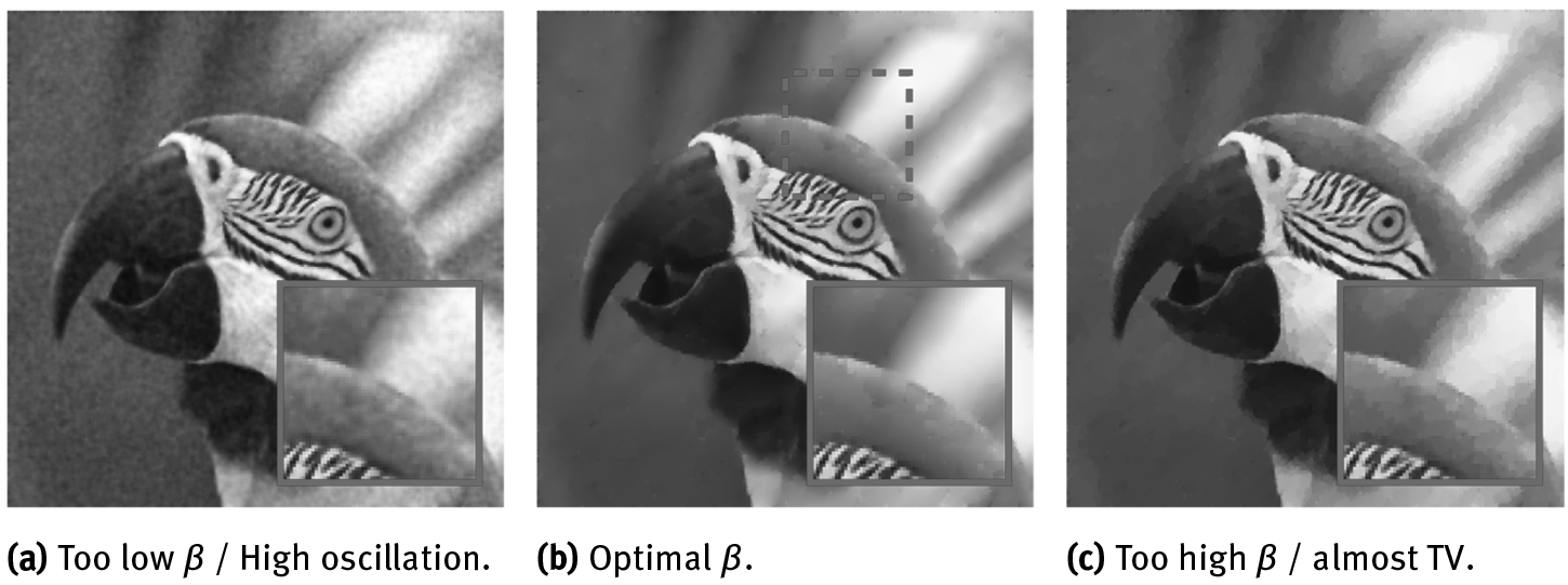
Because one of the main characteristics of images are edges as they define divisions between objects in a scene, the preservation of edges seems like a very good idea and a favorable feature of TV regularization. The drawback of such a regularization procedure becomes apparent as soon as images or signals (in 1D) are considered which do not only consist of constant regions and jumps, but also possess more complicated, higher order structures, for example piecewise linear parts. The artifact introduced by TV regularization in this case is called staircasing [85], compare Figure 3.
One possibility to counteract such artifacts is the introduction of higher order derivatives in the image regularization. Here, we mainly concentrate on two second-order total variation models: the recently proposed Total Generalized Variation (TGV) [9] and the Infimal-Convolution Total Variation (ICTV) model of Chambolle and Lions [25]. We focus on second-order TV regularization only since this is the one that seems to be most relevant in imaging applications [10, 61]. For Ω ⊂ ℝ2 open and bounded, the ICTV regularizer reads

Conversely, second-order TGV [11, 12] reads

Here BD(Ω) := {w ∈ L1(Ω;ℝn) | ‖Ew‖M(Ω;ℝn×n ) < ∞} is the space of vector fields of bounded deformation on Ω, E denotes the symmetrized gradient and Sym2(ℝ2) the space of symmetric tensors of order 2 with arguments in ℝ2. The parameters α, β are fixed positive parameters. The main difference between (4.2) and (4.3) is that we do not generally have that w = ∇υ for any function υ. This results in some qualitative differences of ICTV and TGV regularization, compare for instance [5]. Substituting αR(u) in(1.1) by αTV(u),  gives the TV image reconstruction model, TGV image reconstruction model and the ICTV image reconstruction model, respectively. We observe that in (P) a linear combination of regularizers is allowed and, similarly, a linear combination of data fitting terms is admitted (see Section 8.5.3 for more details). As mentioned already in Remark 2.1, more general bilevel optimization models encoding nonlinear modeling in a finite-dimensional setting have been considered, for instance, in [54] for blind deconvolution and recently in [27, 29] for learning the optimal nonlinear filters in several imaging applications.
8.4.2Optimal parameter choice for TV-type regularization
The regularization effect of TV and second-order TV approaches as discussed above heavily depends on the choice of the regularization parameters α (i.e., (α, β) for second-order TV approaches). In Figures 4 and 5 we show the effect of different choices of α and β in TGV2 denoising. In what follows we show some results from [38] applying the learning approach (Pγ,μ) to find optimal parameters in TV-type reconstruction models, as well as a new application of bilevel learning to optimal cartoon-texture decomposition.

Optimal TV, TGV2 and ICTV denoising
We focus on the special case of K = Id and L2-squared cost F and fidelity term Φ as introduced in Section 8.2.2. In [38, 39] we also discuss the analysis and the effect of Huber regularized L1 costs, but this is beyond the scope of this paper and we refer the reader to the respective papers. We consider the problem for finding optimal parameters (α, β) for the variational regularization model

where f is the noisy image, R(α,β) is either TV in (4.1) multiplied by α (then β is obsolete),  in (4.3) or ICTV(α,β) in (4.2). We employ the framework of (Pγ,μ) witha training pair (f0, f) of original image f0 and noisy image f, using L2-squared cost
 As a first example we consider a photograph of a parrot to which we add Gaussian noise such that the PSNR of the parrot image is 24.72. In Figure 6, we plot by the red star the discovered regularization parameter (α∗, β∗) reported in Figure 7. Studying the location of the red star, we may conclude that the algorithm managed to find a nearly optimal parameter in very few BFGS iterations, compare Table 1.
The figure also indicates a nearly quasi-convex structure of the mapping 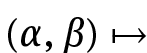
 Although no real quasi-convexity can be proven, this is still suggestive that numerical methods can have good performance. Indeed, in all of our experiments, more of which can be found in the original article [38], we have observed commendable convergence behavior of the BFGS-based algorithm.
Generalizing power of the model
To test the generalizing power of the learning model, we took the Berkeley segmentation data set (BSDS300, [69]), resizing each image to a computationally manageable 128 pixels on its shortest edge, and took the 128 × 128 top-left square of the image. To the images, we applied pixelwise Gaussian noise of variance σ = 10. We then split

 cost functional plotted versus (α, β) for TGV2 denoising. The illustration is a contour plot of function value versus (α, β).
Table 1: Quantified results for the parrot image (ℓ = 256 = image width/height in pixels).


 2
2
the data set into two halves, each of 100 images. We learned a parameter for each half individually, and then denoised the images of the other half with that parameter. The results for TV regularization with L2 cost and fidelity are in Table 2, and for TGV2 regularization in Table 3. As can be seen, the parameters learned using each half, hardly differ. The average PSNR and SSIM, when denoising using the optimal parameter, learned using the same half, and the parameter learned from the other half, also differ insignificantly. We can therefore conclude that the bilevel learning model has good generalizing power.
Optimizing cartoon-texture decomposition using a sketch
It is not possible to distinguish noise from texture by the G-norm and related approaches [70]. Therefore, learning an optimal cartoon-texture decomposition based on a noise image and a ground-truth image is not feasible. What we did instead, is to make a hand-drawn sketch as our expected “cartoon” f0, and then use the bi-level
Table 2: Cross-validated computations on the BSDS300 data set [69] split into two halves, both of 100 images. Total variation regularization with L2 cost and fidelity. “Learning” and “Validation” indicate the halves used for learning α, and for computing the average PSNR and SSIM, respectively. Noise variance σ = 10.

Table 3: Cross-validated computations on the BSDS300 data set [69] split into two halves, both of 100 images. TGV2 regularization with L2 cost and fidelity. “Learning” and “Validation” indicate the halves used for learning α, and for computing the average PSNR and SSIM, respectively. Noise variance σ = 10.

Table 4: Quantified results for cartoon-texture decomposition of the parrot image (ℓ = 256 = image width/height in pixels).
 22
22

framework to find the true “cartoon” and “texture” as split by the model

for the Kantorovich–Rubinstein norm of [64]. For comparison we also include basic TV regularization results, where we define υ = f − u. The results for two different images are in Figure 8 and Table 4, and Figure 9 and Table 5, respectively.

 for KRTV and α⃗ = 0.1/ℓ for TV.
Table 5: Quantified results for cartoon-texture decomposition of the Barbara image (ℓ = 256 = image width/height in pixels).

8.5Learning the data model
The correct mathematical modeling of the data term d in (1.1) is crucial for the design of a realistic image reconstruction model fitting appropriately the given data. Its choice is often driven by physical and statistical considerations on the noise and a Maximum A Posteriori (MAP) approach is frequently used to derive the underlying model. Typically the noise is assumed to be additive, Gaussian-distributed with zero mean and variance σ2 determining the noise intensity. This assumption is reasonable in most of the applications because of the Central Limit Theorem. One alternative often used to model transmission errors affecting only a percentage of the pixels in the image consists in considering a different additive noise model where the intensity values of only a fraction of pixels in the image are switched to either the maximum/ minimum value of the image dynamic range or to a random value within it, with positive probability. This type of noise is called impulse or “salt & pepper” noise. Further, in astronomical imaging applications a Poisson distribution of the noise appears more reasonable, since the physical properties of the quantized (discrete) nature of light and the independence property in the detection of photons show dependence on the signal itself,thus making the use of an additive Gaussian modeling not appropriate.

 for KRTV and α⃗ =0.1/ℓ for TV.
8.5.1Variational noise models
From a mathematical point of view, starting from the pioneering work of Rudin, Osherand Fatemi [89], in the case of Gaussian noise a L2-type data fidelity ϕ(u) = (f − u)2 is typically considered. In the case of impulse noise, variational models enforcing the sparse structure of the noise distribution make use of the L1 norm and have been considered, for instance, in [74]. For those models then ϕ(u) = |f −u|. Poisson noise-based models have been considered in several papers by approximating such distribution with a weighted-Gaussian distribution through variance-stabilizing techniques [15, 93]. In [90] a statistically consistent analytical modeling for Poisson noise distributions has been derived: the resulting data fidelity term is the Kullback–Leibler-type functional ϕ(u) = f − u log u.
As a result of different image acquisition and transmission factors, very often in applications the presence of multiple noise distributions has to be considered. Mixed noise distributions can be observed, for instance, when faults in the acquisition of the image are combined with transmission errors to the receiving sensor. In this case a combination of Gaussian and impulse noise is observed. In other applications, specific tools (such as illumination and/or high-energy beams) are used before the signal is actually acquired. This process is typical, for instance, in microscope and Positron Emission Tomography (PET) imaging applications and may result in a combination of a Poisson-type noise and an additive Gaussian noise. In the imaging community, several combinations of the data fidelities above have been considered for this type of problem. In [52], for instance, a combined L1–L2 TV-based model is considered for joint impulse and Gaussian noise removal. A two-phase approach is considered in [19] where two sequential steps with L1 and L2 data fidelity are performed to remove the impulse and the Gaussian component in the noise, respectively. Mixtures of Gaussian and Poisson noise have also been considered. In [57], for instance, the exact log-likelihood estimator of the mixed model is derived and its numerical solution is computed via a primal-dual splitting, while in other works (see, e.g., [44]) the discrete-continuous nature of the model (because of the Poisson–Gaussian component, respectively) is approximated to an additive model by using homomorphic variancestabilizing transformations and weighted-L2 approximations.
We now complement the results presented in Section 8.2.2 and focus on the choice of the optimal noise models ϕi best fitting the acquired data, providing some examples for the single and multiple noise estimation case. In particular, we focus on the estimation of the optimal fidelity weights λi , i = 1, . . . , M appearing in (P) and (Pγ,μ), which measure the strength of the data fitting and stick with the Total-Variation regularization (4.1) applied to denoising problems. Compared to Section 8.2.1, this corresponds to fixing  and K = Id. We base our presentation on [23, 37], where a careful analysis in term of well-posedness of the problem and derivation of the optimality system in this framework is carried out.
Shorthand notation
In order not to make the notation too heavy, we warn the reader that we will use a shorthand notation for the quantities appearing in the regularized problem (Pγ,μ), that is we will write ϕi(υ) for the data fidelities ϕi(x, υ), i = 1. . . , M and u for uλ,γ,μ, the minimizer of Jγ,μ(⋅; λ).
8.5.2Single noise estimation
We start considering the one-noise distribution case (M = 1) where we aim to determine the scalar optimal fidelity weight λ by solving the following optimization problem:

subject to (compare (3.1))

where the fidelity term ϕ will change according to the noise assumed in the data and the pair (f0, f) is the training pair composed of a noise-free and noisy version of the same image, respectively.
Previous approaches for the estimation of the optimal parameter λ∗ in the context of image denoising rely on the use of (generalized) cross-validation [103] or on the combination of the SURE estimator with Monte Carlo techniques [83]. In the case when the noise level is known there are classical techniques in inverse problems for choosing an optimal parameter λ∗ in a variational regularization approach, foe example the discrepancy principle or the L-curve approach [42]. In our discussion we do not use any knowledge of the noise level but rather extract this information indirectly from our training set and translate it to the optimal choice of λ. As we will see later such an approach is also naturally extendible to multiple noise models as well as inhomogeneous noise.
Gaussian noise
We start considering (5.1) for determining the regularization parameter λ in the standard TV denoising model assuming that the noise in the image is normally distributed and ϕ(u) = (u − f)2. The optimization problem 5.1 takes the following form:

subject to:

For the numerical solution of the regularized variational inequality we use a primal-dual algorithm presented in [53].
As an example, we compute the optimal parameter λ∗ in (5.2) for a noisy image distorted by Gaussian noise with zero mean and variance 0.02. Results are reported in Figure 10. The optimization result has been obtained for the parameter values μ = 1e − 12, γ = 100 and h = 1/177.

In order to check the optimality of the computed regularization parameter λ∗, we consider the 80 × 80 pixel bottom left corner of the noisy image in Figure 10. InFigure 11 the values of the cost functional and of the Signal-to-Noise Ratio SNR = for parameter values between 150 and 1200, are plotted. Also the cost functional value corresponding to the computed optimal parameter λ∗ = 885.5 is shown with a cross. It can be observed that the computed weight actually corresponds to an optimal solution of the bilevel problem. Here we have used h = 1/80 and the other parameters as above.
The problem presented consists in the optimal choice of the TV regularization parameter, if the original image is known in advance. This is a toy example for proof of concept only. In applications, this image would be replaced by a training set of images.

Robust estimation with training sets
Magnetic Resonance Imaging (MRI) images seem to be a natural choice for our methodology, since a large training set of images is often at hand and used to make the estimation of the optimal λ∗ more robust. Moreover, for this application the noise is often assumed to be Gaussian distributed. Let us consider a training database of clean and noisy images. We modify (5.2) as:

subject to the set of regularized versions of (5.2b), for k = 1, . . . , K.
As explained in [23], dealing with large training sets of images and nonsmooth PDE constraints of the form (5.2b) may result is very high computational costs as, in principle, each constraint needs to be solved in each iteration of the optimization loop. In order to overcome the computational efforts, we estimate λ∗ using the Dynamic Sampling Algorithm 1.
For the following numerical tests, the parameters are chosen as follows: μ = 1e − 12, γ = 100 and h = 1/150. The noise in the images has distribution ?(0, 0.005) and the accuracy parameter θ of Algorithm 1, is chosen to be θ = 0.5.
Table 6 shows the numerical ∗values of the optimal parameter λ∗ and ![]() computedvarying N after solving all the PDE constraints and using the Dynamic Sampling algorithm, respectively. We measure the efficiency of the algorithms in terms of the number of the PDEs solved during the whole optimization and we compare the efficiency of solving (5.3) subject to the whole set of constraints (5.2b) with the one where the solution is computed by means of the Dynamic Sampling strategy, observing a clear improvement. Computing also the relative error
computedvarying N after solving all the PDE constraints and using the Dynamic Sampling algorithm, respectively. We measure the efficiency of the algorithms in terms of the number of the PDEs solved during the whole optimization and we compare the efficiency of solving (5.3) subject to the whole set of constraints (5.2b) with the one where the solution is computed by means of the Dynamic Sampling strategy, observing a clear improvement. Computing also the relative error  we also observe a goodlevel of accuracy: the error remains always below 5%. This confirms what was discussed previously in Section 8.3.2, that is the robustness of the estimation of the optimal parameter λ∗ is assessed by selecting a suitable subset of training images whoseoptimal size is validated throughout the algorithm by the check of condition of (3.10)which guarantees an efficient and accurate estimation of the parameter.
Table 6: Optimal λ∗ estimation for large training sets: computational costs are reduced via the Dynamic Sampling Algorithm 1.

Figure 12 shows an example of a database of brain images1together with the optimal denoised version obtained by Algorithm 1 for Gaussian noise estimation.

As a second example, we consider the case of images corrupted by Poisson noise. The corresponding data fidelity in this case is ϕ(u) = u − f log u [90] and requires the additional condition for u to be strictly positive. We enforce this constraint by using a standard penalty method and solve:

where u is the solution of the minimization problem:

where η ≫ 1 is a penalty parameter enforcing the positivity constraint and δ ≪ 1 ensures strict positivity throughout the optimization. After Huber-regularizing the TV term using (2.2), we write the primal-dual form of the corresponding optimality condition for the optimization problem (5.4) similarly as in (3.5) and (3.6):

where ?δ is the active set ?δ := {x ∈ Ω: u(x) < δ}. We then design a modified SSN iteration solving (5.5) similarly as described in Section 8.3.1, see [37, Section 4] for more details. Figure 13 shows the optimal denoising result for the Poisson noise case in correspondence of the value λ∗ = 1013.76.
Spatially dependent weight
We continue with an example where λ is spatially dependent. Specifically, we choose as parameter space V = {υ ∈ H1(Ω) : ∂nu = 0 on Γ} in combination with a TV regularizer and a single Gaussian noise model. For this example the noisy image is distorted nonuniformly: A Gaussian noise with zero mean and variance 0.04 is present on the whole image and an additional noise with variance 0.06 is added on the area marked by a red line.
Since the spatially dependent parameter does not allow one to get rid of the positivity constraints in an automatic way, we solved the whole optimality system by means of the semismooth Newton method described in Section 3, combined with a Schwarz domain decomposition method. Specifically, we decomposed the domain first and applied the globalized Newton algorithm in each subdomain afterwards. The detailed numerical performance of this approach is reported in [30].
The results are shown in Figure 14 for the parameters μ = 1e − 16, γ = 25 and h = 1/500. The values of λ on the whole domain are between 100.0 to 400.0. From the right image in Figure 14 we can see the dependence of the optimal parameter λ∗ on the distribution of noise. As expected, at the high-level noise area in the input image, values of λ∗ are lower (darker area) than in the rest of the image.

8.5.3Multiple noise estimation
We now deal with the case of multiple noise models and consider the following optimization lower level problem:

where the modeling function Ψ combines the different fidelity terms ϕi and weights λi in order to deal with the multiple noise case. The case when Ψ is a linear combination of fidelities ϕi with coefficients λi is the one presented in the general model (P) and (Pγ,μ) and has been considered in [23, 37]. In the following, we present also the case considered in [21, 22] of Ψ being a nonlinear function modeling data fidelity terms in an infimal convolution fashion.
Motivated by some previous work in literature on the use of the infimal-convolution operation for image decomposition, cf. [16, 25], we consider in [21, 22] a variational model for mixed noise removal combining classical data fidelities in such fashion with the intent of obtaining an optimal denoised image thanks to the decomposition of the noise into its different components. In the case of combined impulse and Gaussian noise, the optimization model reads:

where u is the solution of the optimization problem:

where w represents the impulse noise component (and is treated using the L1 norm) and the optimization runs over υ and w, see [22]. We use a single training pair (f0, f) and consider a Huber-regularization depending on a parameter γ for both the TV term and the L1 norm appearing in (5.6). The corresponding Euler–Lagrange equations are:

Again, writing the equations above in a primal-dual form, we can write the modified SSN iteration and solve the optimization problem with BFGS as described in Section 8.3.1.
In Figure 15 we present the results of the model considered. The original image f0 has been corrupted with Gaussian noise of zero mean and variance 0.005 and then a percentage of 5% of pixels has been corrupted with impulse noise. The parameters have been chosen to be γ = 1e4, μ = 1e − 15 and the mesh step size h = 1/312. The computed optimal weights are  and
and  Together with an optimal denoised image, the results show the decomposition of the noise into its sparse and Gaussian components, see [22] for more details.
Gaussian and Poisson noise
We consider now the optimization problem with ϕ1(u) = (u − f)2 for the Gaussian noise component and ϕ2(u) = (u − f log u) for the Poisson one. We aim to determine the optimal weighting (λ1, λ2) as follows:


subject to u be the solution of:

for one training pair (f0, f), where f corrupted by Gaussian and Poisson noise. After Huber-regularizing the Total Variation term in (5.7), we derive (formally) the following Euler–Lagrange equation

with nonnegative Lagrange multiplier α ∈ L2(Ω). As in [90] we multiply the first equation by u and obtain

where we have used the complementarity condition α ⋅ u = 0. Next, the solution u is computed iteratively by using a semismooth Newton-type method combined with the outer BFGS iteration as above.
In Figure 16 we show the optimization result. The original image f0 has been first corrupted by Poisson noise and then Gaussian noise was added, with zero mean and variance 0.001. Choosing the parameter values to be γ = 100 and μ = 1e − 15, the optimal weights  and
and  were computed on a grid with mesh size step h = 1/200.
8.6Conclusion and outlook
Machine-learning approaches in image processing and computer vision have mostly been developed in parallel to their mathematical analysis counterparts, which have variational regularization models at their core. Variational regularization techniquesoffer rigorous and intelligible image analysis –which gives reliable and stable answers that provide us with insight into the constituents of the process and reconstruction guarantees, such as stability and error bounds. This guarantee of giving a meaningful and stable result is crucial in most image processing applications, in biomedical and seismic imaging, in remote sensing and astronomy: provably giving an answer which is correct up to some error bounds is important when diagnosing patients, deciding upon a surgery or when predicting earthquakes. Conversely, machine-learning methods are extremely powerful as they learn from examples and are hence able to adapt to a specific task. The recent rise of deep learning gives us a glimpse of what is possible when intelligently using data to learn from. Today’s (29 April 2015) search on Google on the keyword ‘deep learning image’ just gave 59,800,000 hits. Deep learning is employed for all kinds of image processing and computer vision tasks, with impressive results! The weak point of machine-learning approaches, however, is that they generally cannot offer stability or error bounds, neither provide for most of them understanding about the driving factors (e.g., the important features in images) that led to their answer.

 and
and 
In this paper we wanted to give an account of a recently started discussion in mathematical image processing about a possible marriage between machine learning and variational regularization – an attempt to bring together the good from both worlds. In particular, we have discussed bilevel optimization approaches in which optimal image regularizers and data fidelity terms are learned making use of a training set. We discussed the analysis of such a bilevel strategy in the continuum as well as their efficient numerical solution by quasi-Newton methods, and presented numerical examples for computing optimal regularization parameters for TV, TGV2 and ICTV denoising, as well as for deriving optimal data fidelity terms for TV image denoising for data corrupted with pure or mixed noise distributions.
Although the techniques presented in this article are mainly focused on denoising problems, the perspectives of using similar approaches in other image reconstruction problems (inpainting, segmentation, etc.) are promising [54, 60, 84] or for optimizing other elements in the setup of the variational model [48]. Also the extension of the analysis to color images deserves to be further studied.
Finally, there are still several open questions which deserve to be investigated in the future. For instance, on the analysis side, is it possible to obtain an optimality system for (P) by performing an asymptotic analysis when μ → 0? On the practical side, how should optimality be measured? Are quality measures such as the signal-to-noise ratio and generalizations thereof [102] enough? Should one try to match characteristic expansions of the image such as Fourier or Wavelet expansions [71]? And do we always need a training set or could we use nonreference quality measures [26]?
Acknowledgment: The original research behind this review was supported by the King Abdullah University of Science and Technology (KAUST) Award No. KUK-I1-007-43, the EPSRC grants Nr. EP/J009539/1 “Sparse & Higher-order Image Restoration”, and Nr. EP/M00483X/1 “Efficient computational tools for inverse imaging problems”, the Escuela Politécnica Nacional de Quito under award PIS 12-14 and the MATHAm-Sud project SOCDE “Sparse Optimal Control of Differential Equations”. C. Cao and T. Valkonen were also supported by Prometeo scholarships of SENESCYT (Ecuadorian Ministry of Higher Education, Science, Technology and Innovation).
A data statement for the EPSRC: The data leading to this review publication will be made available, as appropriate, as part of the original publications that this work summarizes.
Bibliography
[1]W. K. Allard. Total variation regularization for image denoising, I. Geometric theory. SIAM J. Math. Anal., 39(4):1150–1190, 2008.
[2]L. Ambrosio, A. Coscia, and G. Dal Maso. Fine properties of functions with bounded deformation. Arch. Ration. Mech. Anal., 139:201–238, 1997.
[3]L. Ambrosio, N. Fusco, and D. Pallara. Functions of Bounded Variation and Free Discontinuity Problems. Oxford University Press, 2000.
[4]F. Baus, M. Nikolova, and G. Steidl. Fully smoothed L1-TV models: Bounds for the minimizers and parameter choice. J. Math. Imaging Vision, 48(2):295–307, 2014.
[5]M. Benning, C. Brune, M. Burger, and J. Müller. Higher-order TV methods—enhancement via Bregman iteration. J. Sci. Comput., 54(2-3):269–310, 2013.
[6]M. Benning and M. Burger. Ground states and singular vectors of convex variational regularization methods. Methods and Applications of Analysis, 20(4):295–334, 2013.
[7]L. Biegler, G. Biros, O. Ghattas, M. Heinkenschloss, D. Keyes, B. Mallick, L. Tenorio, B. van Bloemen Waanders, K. Willcox, and Y. Marzouk. Large-scale inverse problems and quantification of uncertainty, volume 712. John Wiley & Sons, 2011.
[8]J. F. Bonnans and D. Tiba. Pontryagin’s principle in the control of semilinear elliptic variational inequalities. Applied Mathematics and Optimization, 23(1):299–312, 1991.
[9]K. Bredies, K. Kunisch, and T. Pock. Total generalized variation. SIAM J. Imaging Sci., 3:492–526, 2011.
[10]K. Bredies and M. Holler. A total variation-based jpeg decompression model. SIAM J. Imaging Sci., 5(1):366–393, 2012.
[11]K. Bredies, K. Kunisch, and T. Valkonen. Properties of l1-TGV2: The one-dimensional case. J. Math. Anal Appl., 398(1):438–454, 2013.
[12]K. Bredies and T. Valkonen. Inverse problems with second-order total generalized variation constraints. In Proc. SampTA 2011, 2011.
[13]A. Buades, B. Coll, and J.-M. Morel. A review of image denoising algorithms, with a new one. Multiscale Model. Simul., 4(2):490–530, 2005.
[14]T. Bui-Thanh, K. Willcox, and O. Ghattas. Model reduction for large-scale systems with highdimensional parametric input space. SIAM J. Sci. Comput., 30(6):3270–3288, 2008.
[15]M. Burger, J. Müller, E. Papoutsellis, and C.-B. Schönlieb. Total variation regularisation inmeasurement and image space for pet reconstruction. Inverse Problems, 10(10), 2014.
[16]M. Burger, K. Papafitsoros, E. Papoutsellis, and C.-B. Schönlieb. Infimal convolution regularisation functionals on bv and lp spaces. part i: The finite p case. Submitted, 2015.
[17]R. H. Byrd, G. M. Chin, W. Neveitt, and J. Nocedal. On the use of stochastic hessian information in optimization methods for machine learning. SIAM J. Optimiz., 21(3):977–995, 2011.
[18]R. H. Byrd, G. M. Chin, J. Nocedal, and Y. Wu. Sample size selection in optimization methods for machine learning. Math. Program., 134(1):127–155, 2012.
[19]J.-F. Cai, R. H. Chan, and M. Nikolova. Two-phase approach for deblurring images corrupted by impulse plus gaussian noise. Inverse Probl. Imaging, 2(2):187–204, 2008.
[20]J.-F. Cai, B. Dong, S. Osher, and Z. Shen. Image restoration: Total variation, wavelet frames, and beyond. Journal of the American Mathematical Society, 25(4):1033–1089, 2012.
[21]L. Calatroni. New PDE models for imaging problems and applications. PhD thesis, University of Cambridge, Cambridge, United Kingdom, September 2015.
[22]L. Calatroni, J. C. De los Reyes, and C.-B. Schönlieb. A variational model for mixed noise distribution. In preparation.
[23]L. Calatroni, J. C. De los Reyes, and C.-B. Schönlieb. Dynamic sampling schemes for optimal noise learning under multiple nonsmooth constraints. In System Modeling and Optimization, pages 85–95. Springer Verlag, 2014.
[24]V. Caselles, A. Chambolle, and M. Novaga. The discontinuity set of solutions of the tv denoising problem and some extensions. Multiscale Model. Simul., 6(3):879–894, 2007.
[25]A. Chambolle and P.-L. Lions. Image recovery via total variation minimization and relatedproblems. Numer. Math., 76:167–188, 1997.
[26]D. M. Chandler. Seven challenges in image quality assessment: past, present, and future research. ISRN Signal Processing, 2013, 2013.
[27]Y. Chen, W. Yu, and T. Pock. On learning optimized reaction diffusion processes for effective image restoration. In The IEEE Conference on Computer Vision and Pattern Recognition(CVPR), pages 5261–5269, 2015.
[28]Y. Chen, T. Pock, and H. Bischof. Learning ℓ1-based analysis and synthesis sparsity priors using bi-level optimization. In Workshop on Analysis Operator Learning vs. Dictionary Learning, NIPS 2012, 2012.
[29]Y. Chen, R. Ranftl, and T. Pock. Insights into analysis operator learning: From patch-based sparse models to higher-order mrfs. IEEE Trans. Image Process., 23(3):1060–1072, 2014.
[30]C. V. Chung and J. C. De los Reyes. Learning optimal spatially-dependent regularization parameters in total variation image restoration. In preparation.
[31]J. Chung, M. Chung, and D. P. O’Leary. Designing optimal spectral filters for inverse problems. SIAM J. Sci. Comput., 33(6):3132–3152, 2011.
[32]J. Chung, M. I. Español, and T. Nguyen. Optimal regularization parameters for general-form tikhonov regularization. arXiv preprint arXiv:1407.1911, 2014.
[33]A. Cichocki, S.-i. Amari, et al. Adaptive Blind Signal and Image Processing. John Wiley Chichester, 2002.
[34]R. Costantini and S. Susstrunk. Virtual sensor design. In Electronic Imaging 2004, pages 408–419. International Society for Optics and Photonics, 2004.
[35]J. C. De los Reyes. Optimal control of a class of variational inequalities of the second kind. SIAM Journal on Control and Optimization, 49(4):1629–1658, 2011.
[36]J. C. De los Reyes. Numerical PDE-Constrained Optimization. Springer, 2015.
[37]J. C. De los Reyes and C.-B. Schönlieb. Image denoising: Learning the noise model via nonsmooth PDE-constrained optimization. Inverse Probl. Imaging, 7(4), 2013.
[38]J. C. De los Reyes, C.-B. Schönlieb, and T. Valkonen. Bilevel parameter learning for higher-order total variation regularisation models. submitted, 2015.
[39]J. C. De los Reyes, C.-B. Schönlieb, and T. Valkonen. The structure of optimal parameters for image restoration problems. J. Math. Anal. Appl., 434(1):464–500, 2016.
[40]J. Domke. Generic methods for optimization-based modeling. In International Conference on Artificial Intelligence and Statistics, pages 318–326, 2012.
[41]Y. Dong and M. M. Hintermüller, and M. Rincon-Camacho. Automated regularization parameter selection in multi-scale total variation models for image restoration. J. Math. ImagingVision, 40(1):82–104, 2011.
[42]H. W. Engl, M. Hanke, and A. Neubauer. Regularization of Inverse Problems, volume 375. Springer, 1996.
[43]S. N. Evans and P. B. Stark. Inverse problems as statistics. Inverse Problems, 18(4):R55, 2002.
[44]A. Foi. Clipped noisy images: Heteroskedastic modeling and practical denoising. Signal Processing, 89(12):2609 – 2629, 2009. Special Section: Visual Information Analysis for Security.
[45]K. Frick, P. Marnitz, A. Munk, et al. Statistical multiresolution dantzig estimation in imaging: Fundamental concepts and algorithmic framework. Electronic Journal of Statistics, 6:231–268, 2012.
[46]G. Gilboa. A total variation spectral framework for scale and texture analysis. SIAM J. Imaging Sci., 7(4):1937–1961, 2014.
[47]G. Gilboa and S. Osher. Nonlocal operators with applications to image processing. Multiscale Modeling & Simulation, 7(3):1005–1028, 2008.
[48]E. Haber, L. Horesh, and L. Tenorio. Numerical methods for experimental design of large-scale linear ill-posed inverse problems. Inverse Problems, 24(5):055012, 2008.
[49]E. Haber and L. Tenorio. Learning regularization functionals – a supervised training approach. Inverse Problems, 19(3):611, 2003.
[50]E. Haber, L. Horesh, and L. Tenorio. Numerical methods for the design of large-scale nonlinear discrete ill-posed inverse problems. Inverse Problems, 26(2):025002, 2010.
[51]M. Hintermüller, A. Laurain, C. Löbhard, C. N. Rautenberg, and T. M. Surowiec. Elliptic mathematical programs with equilibrium constraints in function space: Optimality conditions and numerical realization. In Trends in PDE Constrained Optimization, pages 133–153. SpringerInternational Publishing, 2014.
[52]M. Hintermüller and A. Langer. Subspace correction methods for a class of nonsmooth and nonadditive convex variational problems with mixed l1/l2 data-fidelity in image processing. SIAM J. Imaging Sci., 6(4):2134–2173, 2013.
[53]M. Hintermüller and G. Stadler. An infeasible primal-dual algorithm for total bounded variation–based inf-convolution-type image restoration. SIAM J. Sci. Comput., 28(1):1–23, 2006.
[54]M. Hintermüller and T. Wu. Bilevel optimization for calibrating point spread functions in blind deconvolution. Preprint, 2014.
[55]H. Huang, E. Haber, L. Horesh, and J. K. Seo. Optimal estimation of L1-regularization prior from a regularized empirical bayesian risk standpoint. Inverse Probl. Imaging, 6(3), 2012.
[56]J. Idier. Bayesian approach to inverse problems. John Wiley & Sons, 2013.
[57]A. Jezierska, E. Chouzenoux, J.-C. Pesquet, and H. Talbot. A Convex Approach for ImageRestoration with Exact Poisson-Gaussian Likelihood. Technical report, December 2013.
[58]J. Kaipio and E. Somersalo. Statistical and computational inverse problems, volume 160. Springer Science & Business Media, 2006.
[59]N. Kingsbury. Complex wavelets for shift invariant analysis and filtering of signals. Applied and Computational Harmonic Analysis, 10(3):234–253, 2001.
[60]T. Klatzer and T. Pock. Continuous Hyper-parameter Learning for Support Vector Machines. InComputer Vision Winter Workshop (CVWW), 2015.
[61]F. Knoll, K. Bredies, T. Pock, and R. Stollberger. Second order total generalized variation (TGV) for MRI. Magnetic Resonance in Medicine, 65(2):480–491, Feb 2011.
[62]V. Kolehmainen, T. Tarvainen, S. R. Arridge, and J. P. Kaipio. Marginalization of uninteresting distributed parameters in inverse problems: application to diffuse optical tomography.International Journal for Uncertainty Quantification, 1(1), 2011.
[63]K. Kunisch and T. Pock. A bilevel optimization approach for parameter learning in variational models. SIAM J. Imaging Sci., 6(2):938–983, 2013.
[64]J. Lellmann, D. Lorenz, C.-B. Schönlieb, and T. Valkonen. Imaging with Kantorovich-Rubinstein discrepancy. SIAM J. Imaging Sci., 7:2833–2859, 2014.
[65]Z.-Q. Luo, J.-S. Pang, and D. Ralph. Mathematical programs with equilibrium constraints. Cambridge University Press, 1996.
[66]J. Mairal, F. Bach, and J. Ponce. Task-driven dictionary learning. IEEE Transactions on Pattern Analysis and Machine Intelligence (PAMI), 34(4):791–804, 2012.
[67]J. Mairal, F. Bach, J. Ponce, G. Sapiro, and A. Zisserman. Discriminative learned dictionaries for local image analysis. CVPR, 2008.
[68]J. Mairal, F. Bach, J. Ponce, and G. Sapiro. Online dictionary learning for sparse coding. InProceedings of the 26th Annual International Conference on Machine Learning, pages 689–696. ACM, 2009.
[69]D. Martin, C. Fowlkes, D. Tal, and J. Malik. A database of human segmented natural images and its application to evaluating segmentation algorithms and measuring ecologicalstatistics. In Proc. 8th Int’l Conf. Computer Vision, volume 2, pages 416–423, July 2001. Thedatabase is available online at http://www.eecs.berkeley.edu/Research/Projects/CS/vision/bsds/BSDS300/html/dataset/images.html.
[70]Y. Meyer. Oscillating patterns in image processing and nonlinear evolution equations. AMS, 2001.
[71]D. Mumford and B. Gidas. Stochastic models for generic images. Quarterly of Applied Mathematics, 59(1):85–112, 2001.
[72]F. Natterer and F. Wübbeling. Mathematical Methods in Image Reconstruction. Monographs on Mathematical Modeling and Computation Vol 5, Philadelphia, PA: SIAM), 2001.
[73]Y. Nesterov. Primal-dual subgradient methods for convex problems. Math. Programm., 120(1):221–259, 2009.
[74]M. Nikolova. A variational approach to remove outliers and impulse noise. J. Math. Imaging Vision, 20(1-2):99–120, 2004.
[75]J. Nocedal and S. Wright. Numerical Optimization. Springer Series in Operations Research and Financial Engineering. Springer, 2006.
[76]P. Ochs, R. Ranftl, T. Brox, and T. Pock. Bilevel Optimization with Nonsmooth Lower LevelProblems. In International Conference on Scale Space and Variational Methods in ComputerVision (SSVM), 2015. to appear.
[77]B. Olshausen and D. Field. Emergence of simple-cell receptive field properties by learning a sparse code for natural images. Nature, 381:607–609, 1996.
[78]J. V. Outrata. A generalized mathematical program with equilibrium constraints. SIAM Journal on Control and Optimization, 38(5):1623–1638, 2000.
[79]K. Papafitsoros and K. Bredies. A study of the one dimensional total generalised variation regularisation problem. arXiv preprint arXiv:1309.5900, 2013.
[80]G. Peyré, S. Bougleux, and L. Cohen. Non-local regularization of inverse problems. In Computer Vision–ECCV 2008, pages 57–68. Springer, 2008.
[81]G. Peyré, S. Bougleux, and L. D. Cohen. Non-local regularization of inverse problems. Inverse Problems and Imaging, 5(2):511–530, 2011.
[82]G. Peyré and J. M. Fadili. Learning analysis sparsity priors. Sampta’11, 2011.
[83]S. Ramani, T. Blu, and M. Unser. Monte-carlo SURE: A black-box optimization of regularization parameters for general denoising algorithms. IEEE Transactions on Image Processing, 17(9):1540–1554, 2008.
[84]R. Ranftl and T. Pock. A deep variational model for image segmentation. In 36th German Conference on Pattern Recognition ( GCPR), 2014.
[85]W. Ring. Structural properties of solutions to total variation regularization problems. ESAIM: Math. Model. Numer. Anal., 34:799–810, 7 2000.
[86]H. Robbins and S. Monro. A stochastic approximation method. Ann. Math. Statist., 22(3):400–407, 1951.
[87]R. T. Rockafellar and R. J.-B. Wets. Variational Analysis. Springer, 1998.
[88]S. Roth and M. J. Black. Fields of experts: A framework for learning image priors. In ComputerVision and Pattern Recognition, 2005. CVPR 2005. IEEE Computer Society Conference on, volume 2, pages 860–867. IEEE, 2005.
[89]L. I. Rudin, S. Osher, and E. Fatemi. Nonlinear total variation based noise removal algorithms. Physica D: Nonlinear Phenomena, 60(1):259–268, 1992.
[90]A. Sawatzky, C. Brune, J. Müller, and M. Burger. Total variation processing of images withpoisson statistics. In Xiaoyi Jiang and Nicolai Petkov, editors, Computer Analysis of Images and Patterns, volume 5702 of Lecture Notes in Computer Science, pages 533–540. Springer Berlin Heidelberg, 2009.
[91]L. L. Scharf. Statistical Signal Processing, volume 98. Addison-Wesley Reading, MA, 1991.
[92]U. Schmidt and S. Roth. Shrinkage fields for effective image restoration. In Computer Vision and Pattern Recognition (CVPR), 2014 IEEE Conference on, pages 2774–2781. IEEE, 2014.
[93]J.-L. Starck, F. D. Murtagh, and A. Bijaoui. Image restoration with noise suppression using awavelet transform and a multiresolution support constraint. Proc. SPIE, 2302:132–143, 1994.
[94]E. Tadmor, S. Nezzar, and L. Vese. A multiscale image representation using hierarchical (BV, L2) decompositions. Multiscale Model. Simul., 2(4):554–579, 2004.
[95]Marshall F Tappen. Utilizing variational optimization to learn Markov random fields. In Computer Vision and Pattern Recognition, 2007. CVPR’07. IEEE Conference on, pages 1–8. IEEE,2007.
[96]R. Temam. Mathematical problems in plasticity. Gauthier-Villars, 1985.
[97]M. Unser. Texture classification and segmentation using wavelet frames. Image Processing, IEEE Transactions on, 4(11):1549–1560, 1995.
[98]M. Unser and N. Chenouard. A unifying parametric framework for 2d steerable wavelet transforms. SIAM J. Imaging Sci., 6(1):102–135, 2013.
[99]T. Valkonen. The jump set under geometric regularisation. Part 1: Basic technique and first-order denoising. SIAM J. Math. Anal., July 2015. Accepted.
[100]Y. Vardi, L. A. Shepp, and L. Kaufman. A statistical model for positron emission tomography. Journal of the American Statistical Association, 80(389):8–20, 1985.
[101] F. Viola, A. Fitzgibbon, and R. Cipolla. A unifying resolution-independent formulation for early vision. In Computer Vision and Pattern Recognition (CVPR), 2012 IEEE Conference on, pages494–501. IEEE, 2012.
[102]Z. Wang, A. C. Bovik, H. R. Sheikh, and E. P. Simoncelli. Image quality assessment: From errorvisibility to structural similarity. IEEE Trans. Image Processing, 13(4):600–612, 2004.
[103]N. Weyrich and G. T. Warhola. Wavelet shrinkage and generalized cross validation for imagedenoising. IEEE Transactions on Image Processing, 7(1):82–90, 1998.
[104]G. Yu, G. Sapiro, and S. Mallat. Image modeling and enhancement via structured sparse model selection. Proc. IEEE Int. Conf. Image Processing, 2010.