Jérôme Lohéac and Jean-François Scheid
15Time-optimal controlfor a perturbed Brockett integrator
Jérôme Lohéac, LUNAM Université, IRCCyN UMR CNRS 6597 (Institut de Recherche en Communications et Cybernétique de Nantes), École des Mines de Nantes, 4 rue Alfred Kastler, 44307 Nantes,France, [email protected]
Jean-François Scheid, IECL – Institut Élie Cartan de Lorraine, UMR 7502, Université de Lorraine, Campus des Aiguillettes, B.P. 70239, 54506 Vandoeuvre-lès-Nancy Cedex, France, [email protected]
Application to time-optimal axisymmetric micro-swimmers
Abstract: The aim of this paper is to compute time-optimal controls for a perturbation of a Brockett integrator with state constraints. Brockett integrator and its perturbations appear in many application fields. One of them described in details in this paper is the swimming of micro-organisms. We present some key results for a fast and robust numerical method to compute time-optimal controls for the perturbation of a Brockett integrator. This numerical method is based on explicit formulae of time-optimal controls for the Brockett integrator. The methodology presented in this paper is applied to the time-optimal control of a micro-swimmer.
Keywords: Time-optimal controllability, Brockett integrator, state constraints, numerical resolution, micro-swimmers
AMS classification: 34H05, 49J15, 49K15, 49K20, 93C15
15.1Introduction
In this section, we consider the following system:

where (h, α) ∈ ℝ × ℝn are the state variables, λ ∈ ℝn is the control variable, and V : ℝn → ℝn is a given map. In (1.1a), ⟨⋅, ⋅⟩ denotes the Euclidean product in ℝn. The system (1.1a), (1.1b) is completed with the initial conditions:

The first aim of this section is the following. Given T > 0, hf ∈ ℝ∗, and c > 0, find a control λ : [0, T] → ℝn such that the final target hf is reached at time T:

together with the state constraint:

where | ⋅ | denotes the Euclidean norm in ℝn.
Providing that V ∈ C∞(ℝn, ℝn) and the Jacobian matrix ∇V(0) ∈ Mn(ℝ) is not symmetric, we prove that this control problem can be solved. More precisely, there exists a minimal time T⋆ = T⋆(hf , c) > 0 such that the control problem (1.1)–(1.3) admits a solution λ ∈ BV([0, T], ℝn) together with the control constraint:

The second aim of this section, which actually constitutes the main issue of this paper, is to present an efficient numerical method for the computation of time-optimal controls for the system (1.1)–(1.4). The method relies on explicit optimal solutions given in [22] for the time-optimal control problem (1.1)–(1.4) with V(α) = Mα where M ∈ M n(ℝ) is a nonsymmetric matrix. The numerical method is also based on a full direct discretization as depicted in [30, § 9.II.1]. Let us mention that (1.1) with V(α) = Mα is a natural extension of the Brockett integrator:
ḣ = α2λ1 − α1λ2 ,
α̇1 = λ1 ,
α̇2 = λ2 .
Roughly speaking, up to some adaptations, our numerical method is a full direct discretization method (see [30, § 9.II.1]) initialized with the analytic solution obtained in [22] for M = ∇V(0). Numerical examples will show that this initialization procedure provides better results than arbitrary initial guesses. It improves the robustness and reduces the computational time.
This strategy is applied to the time-optimal control of micro-swimmers. We will see that the efficiency of the micro-swimmer we consider is low and the minimal time is high. Our strategy also provides a preliminary estimate of the minimal control time and hence we also get an estimate of the time discretization step required for suitable results. In this note, we only focus on numerical results. No theoretical proof of robustness nor algorithmic complexity are given. We emphasize that even if direct discretizationmethods are robust for control problems, knowing an approximation of the optimal solution is even better.
Moreover, in this paper, for the sake of clarity, we only present the dimension case n = 2, but a similar methodology can be obtained for any n ≥ 2.
This paper is organized as follows. We first give controllability and time-optimal controllability results for the control problem (1.1)–(1.4) in Section 15.2. Analytic results obtained in [22] are recalled in Section 15.3. In Section 15.4, we present the numerical strategy and its application to time-optimalmicro-swimmers is studied in Section 15.5.
15.2Controllability and time-optimal controllability
Using Chow theorem, the following controllability result holds.
Proposition 2.1. Let c > 0 and V ∈ C∞(ℝ2, ℝ2) be given and assume that the Jacobian matrix ∇V(0) is not symmetric, that is,
Then, for every hf ∈ ℝ∗ and every T > 0, there exists λ ∈ C0([0, T], ℝ2) with |λ(t)| ≤ 1 for all t ∈ [0, T] such that the solution of (1.1) satisfies the final condition (1.2) together with the state constraint (1.3).
Proof. Let us write f1(h, α) = (V1(α), 1, 0)⊤ and f2(h, α) = (V2(α), 0, 1)⊤ for V(α) = (V1(α), V2(α))⊤. The system (1.1) becomes

The Lie bracket of f1 and f2 at the point 0 is given by

which does not vanish if ∇V(0) is not a symmetric matrix. Thus, under this assumption, the Lie algebra generated by {f1, f2} and evaluated at the point 0 is of dimension 3. In addition, this Lie algebra is independent of h and the fist-order Lie bracket is continuous with respect to α. Therefore, there exists ε > 0 such that for every (h, α) ∈ ℝ×B0(ε), the Lie algebra generated by {f1, f2} evaluated at the point (h, α) is of dimension 3.
The result follows from Chow’s theorem (see for instance [30, Chap. 5, Proposition 5.14], [1] or [17]).
This result combined with the Filippov theorem (see for instance [1, 10, 16]) leads to the following optimal control result.
Proposition 2.2. Let c > 0 and V ∈ C∞(ℝ2, ℝ2) such that ∇V(0) ≠ (∇V(0))⊤. Then, theset of times T > 0 such that there exists λ ∈ BV(0, T)2 with |λ(t)| ≤ 1 for almost every time t ∈ [0, T] and such that the solution (h, α) of (1.1) satisfies the final condition (1.2) together with the state constraint (1.3) on α, admits a minimum value T⋆ = T⋆(hf , c) > 0.
Remark 2.3.
- The constraint |λ(t)| ≤ 1 on the control variable λ is necessary to make the timeminimal control problem relevant. Without this constraint, one can build a sequence of time
 and associated controls λn ∈ BV(0, Tn)2 solving thecontrol problem such that Tn → 0. Thus, the corresponding time-optimal control does not make sense.
 - As in [22, Proposition 3.3], it can be proved that if λ is a time-optimal control, then |λ(t)| = 1 for almost every t ∈ [0, T⋆]. Consequently, the control variable can be written as λ(t) = R(Θ(t))e1 for almost every t, with Θ(t) ∈ ℝand

denotes the rotation matrix of angle θ.
15.3An approximate linearized time-optimal control problem
For a small parameter c > 0, we have V(α) = V(0) + ∇V(0)α + o(c) for every α ∈ B0(c). Instead of considering the time-optimal controllability of the system (1.1), we first consider the approximated linear system:

with the initial condition (1.1c).
We assume that the Jacobian matrix of V at α = 0 is not symmetric. Thus, Proposition 2.2 ensures the existence of a minimal time T⋆ such that the solution (h, α, λ) of the control problem (3.1) with initial condition (1.1c) satisfies (1.2) together with (1.3) and (1.4). In addition, according to [22, Proposition 7], this optimal time T⋆ and time-optimal controls can be explicitly computed.
Proposition 3.1. Let hf ≠ 0, c > 0, and V ∈ C∞(ℝ2, ℝ2). Let γ ∈ ℝ such that γJ =(∇V(0) − (∇V(0))⊤) with  . Assume γ ≠ 0 and define

Then, the minimal time T⋆ of the control problem (3.1), (1.1c), (1.2), (1.3), and (1.4) is given by

Moreover, the time-optimal control λ⋆ is continuous and given by

where, for every θ ∈ ℝ, R(θ) is the rotation matrix of angle θ defined by (2.1), Θ0 is anyreal constant, and Θ(t) is given by the following


Proof. Since α(0) = α(T), it can be easily proved that λ is a control on [0, T] for thesystem (3.1), (1.1c)–(1.4) if and only if λ is a control on [0, T] for the following system:

together with (3.1), (1.1c)–(1.4). The result follows from [22, Proposition 7].
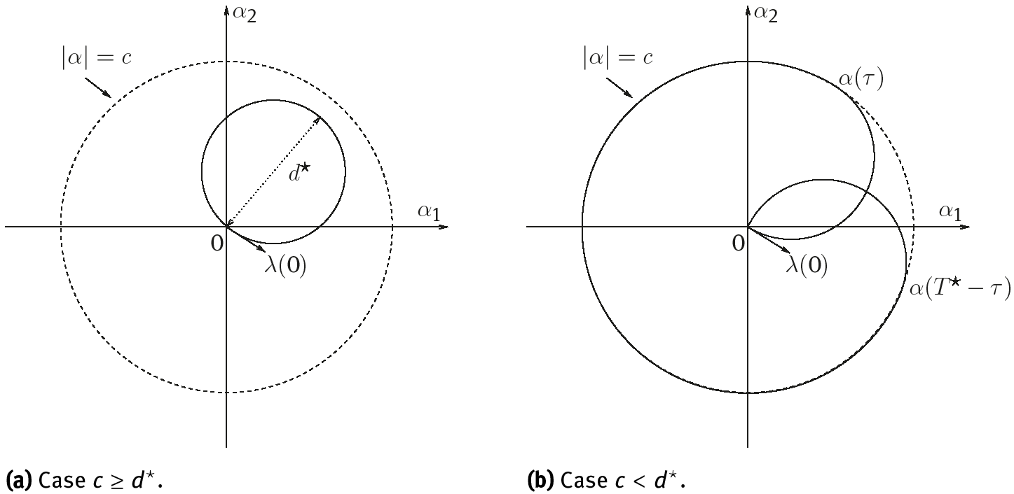
Remark 3.2. Let us explain the formulae of the optimal solution given in Proposition 3.1. The optimal deformation  ds possesses the following characteristics (see Figure 1):
–Ifc ≥ d⋆, the optimal trajectory t → α⋆(t) is a circle of diameter d⋆, starting from 0;
–ifc < d⋆, the optimal trajectory t → α⋆(t) is composed of three arcs of circle. The first arc of circle is a half-circle of diameter c, starting from 0. The second one lies on the circle of diameter 2c, centered at the origin 0. Finally, the third arc of circle is a half-circle of diameter c, reaching the origin 0 at the final time t = T⋆.
15.4Numerical computation of a time-optimal trajectory
In this section, we will explain our numerical approach for computing optimal trajectories, which is mainly inspired from [30, § 9.II.1].
15.4.1Finite-dimensional minimization problem
Let us rewrite our time-optimal control problem as a general optimization problem. First of all, we consider a time control T ̄ (i.e., a time that solves the control problem (1.1)–(1.4)) so that the minimal time T⋆ is lower than T ̄ and we define the cost function J0 : (T, λ) ∈ [0, T̄ ]× BV(0, T̄ )2 ↦ T ∈ ℝ. The optimization problem reads as follows:

According to item 2 of Remark 2.3, any optimal solution λ satisfies |λ(t)| = 1 for almost every t and hence it can be expressed as λ(t) = R(Θ(t))e1 for almost every t, with e1 = (1, 0)⊤. The state variable α is also given by  Then,we introduce the new cost function J1 : (T, Θ) ∈ [0, T̄ ]× BV(0, T) → T ∈ ℝ and theabove optimization problem can be simplified to

In order to numerically tackle this problem, we set n ∈ ℕ∗ an integer and t0 < ⋅ ⋅⋅ < tn n + 1 time discretization points. For every i ∈ {0, . . . , n}, we consider Θi ∈ ℝan approximation of Θ(ti). Let us also define a quadrature formula ?(t0, . . . , tk; f0, . . . , fk)approximating
Thus, defining the cost function Jn : (T, Θ0, . . . , Θn) ∈ ℝ+ × ℝn+1 ↦ T ∈ ℝ, the discretized version of (4.1) is

This nonlinear minimization problem can be solved, for instance, with an interiorpoint method, sequential quadratic programming (SQP), or an active-set algorithm (e.g., [7, 9, 13]) as implemented is the Optimization toolbox of MATLAB through the fmincon function. We will see on practical examples that even if the interior point algorithm is robust with respect to the initialization, the better the initialization guess is, the better the result is.
A natural initialization procedure is to use the time-optimal control obtained analytically for the linearized problem with ∇V(0)α in place of V(α).
15.4.2Numerical example
Let us consider the following:

For the computation of the integrals in theminimization problem, we use the trapeze method, that is, for f ∈ C([τ0, τ1], ℝ), we approximate  dt by
dt by

with 
In order to numerically solve the optimization problem (4.2) with (4.3), we use the fmincon function of the Optimization toolbox of MATLAB with a SQP algorithm. A first observation is that if we choose the initial value (T, Θ0, . . . , Θn) = (1, 0, . . . , 0), the algorithm is not converging. On the other hand, when initializing with the optimal solution of the approximate linearized problem(3.1),(1.1c),(1.2)–(1.4) (see Section 15.3), we obtain a reasonable solution to the nonlinear optimization problem(4.2) (Figure 2).
The SQP algorithm with the trivial initialization point, (T, Θ0, . . . , Θn) = (1, 0, . . . ,0), fails to converge because the discrete state trajectory α0, . . . , αn associatedto this control does not fill the state constraint |αk| ≤ c in (4.2). Indeed, for the initial value (T, Θ0, . . . , Θn) = (1, 0, . . . , 0), due to (4.4) we have αk = tke1 for all k ∈ {1, . . . , n} and in particular we get |αn| = |Te1| = T = 1. A way to avoid this is to use the initialization point:


so that the discrete state variables associated to this control are given by αk = 0 (for every k ∈ {0, . . . , n}) and thus the state constraints are satisfied. We compare in Table 1 the solutions obtained for these to different types of initialization values. These results show that the algorithm is more efficient when the optimal solution of the linearized problem is chosen as an initial guess.
In Table 1, the comparison is made with V given by (4.3), the target hf = 1 and the state constraint given by (1.3) with c = 0.3. The number of discretization points is given by n +1, T⋆ is the optimal time obtained, N SQP is the number of iterations inside the SQP algorithm and TCPU returns the CPU time used for computations.
Table 1: Comparison of the results for the two different types of initializations with the SQP algorithm.
(a) Initialization with the initial value (4.5)

(b) Initialization with the optimal control obtained for the linearized problem (3.1)


In addition, the optimal solution for the nonlinear optimization problem (4.2) obtained with the initial value (4.5) does not look as good as the optimal solution obtained from the optimal solution of the linearized problem (3.1) (see in comparison Figures 2 and 3).
15.5Application to time-optimal micro-swimmers
Understanding the motion of micro-organisms is a challenging issue since at their size the fluid forces are only viscous forces and micro-organisms live in a world where inertia does not exist. Despite the pioneer works on modeling and analyzing the motions of micro-swimmers (see for instance [11, 18, 19, 25, 27–29]), the swimming of microorganisms has only been recently tackled as a control problem. A lot of controllability results for various swimmers has been obtained (see for instance [4, 5, 23, 24, 26] for axisymmetric swimmers, [3, 21] for general swimmers, or [6, 12] when the fluid domain is not the whole space ℝ3).
Let us also point out that numerical strategy for axisymmetric swimmers has already been presented in [2]. The work explained in this paper can be seen as an improvement of this numerical strategy when the cost function is reduced to the final time.
In this section, we consider a micro-swimmer performing axisymmetric deformations. We denote by (e1, e2, e3) the canonical basis of ℝ3 and we assume that e1 represents the symmetry axis. At any time, the swimmer will be diffeomorphic to the unit sphere of ℝ3 and its shape at rest is the unit sphere S0.The control problem is the following: starting from the initial location 0, reach the final position hf e1 by shape changes such that at the initial and final positions, the swimmer is the unit sphere of ℝ3.
For those swimmers, we will study the time-optimal controllability of the dynamical system associated to the swimming problem.
15.5.1Modeling and problem formulation
Axisymmetric coordinates
Since we are considering axisymmetric swimmers, we introduce the spherical coordinate system (r, θ, ϕ) ∈ ℝ+× [0, π] × [0, 2π). For every x = (x1 x2 x3)⊤ ∈ ℝ3, the spherical coordinates (r, θ, ϕ) = (r(x), θ(x), ϕ(x)) are such that


with the associated local system of unit vectors (er , eθ, eϕ) given by (see Figure 4)

Swimmer’s deformations
The shape of the swimmer at rest is the unitball ofℝ3 ,which forms the reference shape denoted by S0.We assume that the deformation of the swimmer is axisymmetric with respect to the symmetry axis e1. More precisely, we assume that the deformation X is built from two elementary deformations D1 and D2, that is,

where D1 and D2 are axisymmetric and radial deformations, that is,

with δi ∈ C1([0, π], ℝ) and αi ∈ L∞(ℝ+, ℝ) such that

so that X(t, ⋅) is a C1-diffeomorphism on S0. In practice, we will consider c > 0 small enough such that (1.3) implies (5.3). We define the domain ?(t) occupied by the deformed swimmer at time t in the reference frame attached to the swimmer:
We also assume that the deformation X does not produce any translation. To this end, we introduce the mass density ρ0(x) = 1 in the shape of the swimmer S0 at rest and we assume that the mass is locally preserved during the deformation, that is, to say that the density of the swimmer at any time t ≥ 0 is given by

where JacX(t, ⋅) denotes the Jacobian of the mapping X (t, ⋅). According to (5.1) and (5.2) we have

With this mass density, we have, for all t ≥ 0

and the mass center of the swimmer is given by

Consequently, we assume

so that the mass center of the swimmer does not move with the deformation X.
Finally, let us consider the domain ?†(t) occupied by the swimmer in the fluid at time t ≥ 0, which is given by

Since we have assumed that the deformation X does not introduce any translation,h(t)e1 is the mass center position of the swimmer in the fluid domain at time t. Thedomains S0, ?(t), and ?†(t) are depicted in Figure 5.
In terms of the control theory, α = (α1, α2)⊤ is the system’s input and h is its outputwe aim to control.

Micro-swimmer and fluid flow
It is well known that the system governing the motion of a micro-swimmer is inertia less (see for instance [20, § 5.3] or [11]) and reduced to the following problem coupling:
–the Stokes equation:

where ℱ(t) = ℝ3 ?(t) and with

–the boundary condition (continuity of the velocity at the boundary of the microswimmer):

–quasi-static Newton law:

where  pI3 is the Cauchystress tensor.
The well posedness of (5.7) follows from [14], where the limit (5.7c) has to be understood in a weak sense (i.e.,  More precisely, we have (u, p) ∈
 where we have set

This ensures that  and consequently, theexpression ∫∂S(t)σ(u, p)n dΓ is seen as a duality product (since σ(u, p)n ∈
  (∂?(t))3 and 1 ∈
![]() (∂?(t))).
(∂?(t))).
Let us first notice that in the full system (5.7)–(5.9) the time does not appear directly but only through the parameter α(t). Consequently, we define ?(α) as the image of S0 by the map X(α) : x ∈ ℝ3 ↦ x + α1D1(x) + α2D2(x) ∈ ℝ3, for α ∈ ℝ2 such that (5.3) holds. For convenience, we also define the corresponding fluid domain ℱ(α) = ℝ3 ?(α).
For every α ∈ ℝ2 satisfying (5.3), we define  the solution of

and for i ∈ {1, 2},  is the solution of:

Then, by decomposing the solution (u(t, ⋅), p(t, ⋅)) of (5.7)–(5.8) in terms of 
 and due to the linearity of the Cauchy stress tensor, relation (5.9) becomes

where for every i ∈ {0, 1, 2} and every α ∈ ℝ2 satisfying (5.3), we have set

with 
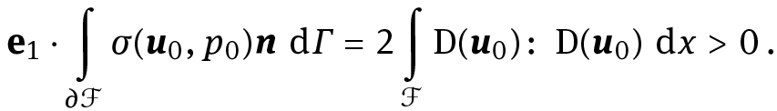
By Green formula, we have
Consequently, F0(α) ⋅ e1 ≠ 0 and the control problem can be recast as the generalizedBrockett system (1.1) with

This system form has already been established in the pioneer work of Alouges et al. [5].Notice that even if α represents the physical control of the swimming system, it is ofmore convenience for analysis to consider λ = α̇ as the control variable. This will also allow us to control both the shape and the position of the swimmer.
We also set the initial conditions (1.1c) for this system and the target position to be reached in a time T > 0 is given by (1.2). These initial and final conditions mean that the micro-swimmer is the unit sphere located at the origin at initial time and a unit sphere located in hf e1 at final time T.
We point out that a state constraint on α is needed to be able to well define Fi(α(t)) for every time t ≥ 0. This constraint is given by (5.3).
In addition, according to [21, Lemma 1] or [23, Theorem 2.6], there exists c > 0 small enough such that the mapping α ∈ ℝ2 ↦ V(α) ∈ ℝ2 with V defined by (5.14) is of regularity C∞ on B0(2c). Consequently, we chose c > 0 small enough such that this condition holds together with (5.3).
Remark 5.1. From [23], there exists δ1, δ2 ∈ C1([0, π], ℝ) in (5.3) such that ∇V(0) is not symmetric. Moreover, using the arguments of [21], this situation is generic.
15.5.2Numerical computation of a time-optimal trajectory
Let us consider the deformations D1 and D2 similar to the one given in [23], that is, to say that D1 and D2 are given by (5.2) with

where P2 (resp. P3) is the Legendre polynomial of order 2 (resp. 3). With these two elementary deformations, we obtain from [27],

These expressions allow us to compute the explicit form of the time-optimal controls for the approximate linearized system (3.1).
In order to numerically compute the fluid forces Fi(α) ⋅ e1 for i ∈ {0, 1, 2}, we use the spherical harmonics expansion of the exterior Stokes solution given in [8] (see also [15] or [27]). Then, we compute the time-optimal controls by using the direct discretizationmethod explained in Section 15.4. The initial guess for the discrete nonlinear optimization problem is chosen as the explicit optimal solution of the approximate linear control problem (3.1) given in Proposition 3.1. We expect that the approximate optimal deformation for the linearized problem is close to the optimal solution for the nonlinear problem so that the direct method will converge quickly.
We apply this computational method with the deformation D1 and D2 given abovethrough Legendre polynomials and we choose c = 0.3 and  The optimal trajectories for h and α are depicted in Figure 6. The optimal time is T⋆ ≃ 48.9.


We numerically observe in Figure 6 that the optimal trajectory for α is mainly periodic. In Figure 7, we also give the optimal trajectory of h during a period in time and finally we plot in Figure 8 the different shapes of the swimmer under the optimal deformation for different instants in the time period.


15.6Conclusion
In this paper, we have presented a numerical strategy for solving a time-minimal control problem for a nonlinear system, which generalizes the Brockett integrator. This method is based on the explicit computation of time-optimal controls for a state constraint Brockett system, which approximates the original nonlinear control problem. These explicit solutions are used as initial guesses in the nonlinear problem. Numerical tests have shown the good behavior of this strategy. This numerical method is then applied to a time-optimal control problem for micro-swimmer with shape changes. The shapes of the swimmer are small deformations of the unit sphere. Despite two elementary deformations are used for the swimmer’s shapes, it is easy to extend this work to the case of a finite number of elementary deformations.
Finally, we observe numerically that the optimal trajectory for α is mainly periodic. It would be interesting to prove rigorously this property. For instance, one could expect the following result: for |hf | large enough and for α ∈ A with A a compact set of ℝ2, the trajectory of α is composed by one starting curve followed by a periodic curve and ending with a final curve. Such a result would be a real improvement for numerical computations since we would only have to solve three simpler (but coupled) time-optimal control problems.
Bibliography
[1]A. A. Agrachev and Y. L. Sachkov. Control theory from the geometric viewpoint, volume 87 of Encyclopaedia of Mathematical Sciences. Springer-Verlag, Berlin, 2004. Control Theory and Optimization, II.
[2]F. Alouges, A. Desimone, and L. Heltai. Numerical strategies for stroke optimization of axisymmetric microswimmers. Math. Models Methods Appl. Sci., 21(2):361–387, 2011.
[3]F. Alouges, A. DeSimone, L. Heltai, A. Lefebvre-Lepot, and B. Merlet. Optimally swimming Stokesian robots. Discrete Contin. Dyn. Syst., Ser. B, 18(5):1189–1215, 2013.
[4]F. Alouges, A. Desimone, and A. Lefebvre. Optimal strokes for low Reynolds number swimmers: An example. J. Nonlinear Sci., 18(3):277–302, 2008.
[5]F. Alouges, A. DeSimone, and A. Lefebvre. Optimal strokes for axisymmetric microswimmers. The European Physical Journal E, 28(3):279–284, 2009.
[6]F. Alouges and L. Giraldi. Enhanced controllability of low Reynolds number swimmers in the presence of a wall. Acta Appl. Math., 128(1):153–179, 2013.
[7]J. F. Bonnans, J.C. Gilbert, C. Lemaréchal, and C.A. Sagastizábal. Numerical optimization. Universitext. Springer-Verlag, Berlin, second edition, 2006. Theoretical and practical aspects.
[8]H. Brenner. The stokes resistance of a slightly deformed sphere. Chemical Engineering Science, 19(8):519 – 539, 1964.
[9]R. H. Byrd, M. E. Hribar, and J. Nocedal. An interior point algorithm for large-scale nonlinear programming. SIAM J. Optim., 9(4):877–900, 1999. Dedicated to John E. Dennis, Jr., on his 60th birthday.
[10]L. Cesari. Optimization—theory and applications, volume 17 of Applications of Mathematics(New York). Springer-Verlag, New York, 1983. Problems with ordinary differential equations.
[11]S. Childress. Mechanics of swimming and flying, volume 2 of Cambridge Studies in Mathematical Biology. Cambridge University Press, Cambridge, 1981.
[12]D. Gérard-Varet and L. Giraldi. Rough wall effect on micro-swimmers. Sept. 2013.
[13]P. E. Gill, W. Murray, and M. H. Wright. Practical optimization. Academic Press, Inc., London-New York, 1981.
[14]V. Girault and A. Sequeira. A well-posed problem for the exterior Stokes equations in two and three dimensions. Arch. Rational Mech. Anal., 114(4):313–333, 1991.
[15]J. Happel and H. Brenner. Low Reynolds number hydrodynamics with special applications to particulate media. Prentice-Hall Inc., Englewood Cliffs, N.J., 1965.
[16]R. F. Hartl, S. P. Sethi, and R. G. Vickson. A survey of the maximum principles for optimal control problems with state constraints. SIAM Rev., 37(2):181–218, 1995.
[17]V. Jurdjevic. Geometric control theory, volume 52 of Cambridge Studies in Advanced Mathematics. Cambridge University Press, Cambridge, 1997.
[18]J. Lighthill. Mathematical biofluiddynamics. Society for Industrial and Applied Mathematics,Philadelphia, Pa., 1975. Based on the lecture course delivered to the Mathematical Biofluiddynamics Research Conference of the National Science Foundation held from July 16–20, 1973, at Rensselaer Polytechnic Institute, Troy, New York, Regional Conference Series in Applied Mathematics, No. 17.
[19]M. J. Lighthill. On the squirming motion of nearly spherical deformable bodies through liquids at very small Reynolds numbers. Comm. Pure Appl. Math., 5:109–118, 1952.
[20]J. Lohéac. Time optimal control and low Reynolds number swimming. Theses, Université de Lorraine, Dec. 2012.
[21]J. Lohéac and A. Munnier. Controllability of 3D low Reynolds number swimmers. ESAIM, Control Optim. Calc. Var., 20(1):236–268, 2014.
[22]J. Lohéac and J.-F. Scheid. Time optimal control for a nonholonomic system with state constraint. Math. Control Relat. Fields, 3(2):185–208, 2013.
[23]J. Lohéac, J.-F. Scheid, and M. Tucsnak. Controllability and time optimal control for low reynolds numbers swimmers. Acta Applicandae Mathematicae, 123:175–200, 2013.
[24]S. Michelin and E. Lauga. Efficiency optimization and symmetry-breaking in a model of ciliary locomotion. Physics of fluids, 22:111901, 2010.
[25]E. Purcell. Life at low Reynolds number. American Journal of Physics, 45:3–11, June 1977.
[26]J. San Martin, T. Takahashi, and M. Tucsnak. A control theoretic approach to the swimming of microscopic organisms. Q. Appl. Math., 65(3):405–424, 2007.
[27]A. Shapere and F. Wilczek. Efficiencies of self-propulsion at low Reynolds number. J. Fluid Mech., 198:587–599, 1989.
[28]A. Shapere and F. Wilczek. Geometry of self-propulsion at low Reynolds number. J. Fluid Mech., 198:557–585, 1989.
[29]G. Taylor. Analysis of the swimming of microscopic organisms. Proc. Roy. Soc. London. Ser. A., 209:447–461, 1951.
[30]E. Trélat. Contrôle optimal. Mathématiques Concrètes. [Concrete Mathematics]. Vuibert, Paris, 2005. Théorie & applications. [Theory and applications].