On the contrary, when the defect in the image is small compared to the patch size, it is possible that the algorithm recovers the structure with just one iteration as is shown in Figure 14. This is also possible, when the initial inpainting function u0 is already close to solution in the sense, that any point in the inpainting domain has enough reliable information within the patch around it.
The patch size also heavily influences the ability of exemplar-based inpainting methods to recover structures. To grasp this issue, we consider an example on a synthetic image and show, that the patch size should not be chosen too small in comparison tothe texture. The problem, which can occur when the patch size is chosen too small, is that a repetitive texture can not be reproduced, as can be seen in Figure 15.

 17 and a Gaussian parameter of σ = 0.1d were used.

Conversely, a too large patch size will first of all increase the computation time. Secondly, large patches might contain too many details and it might be difficult to find suitable exemplars. Without suitable exemplars, it becomes more difficult to recover the structure and the algorithm might even fail to do so. We recall, that in the case of lacking exemplars the behavior of the algorithm is not well understood.
Let us close the analysis of the influence of the patch size by showing results obtained by the patch non-local means scheme applied to the inpainting problem depicted in Figure 15b started with an initialization function u0 that is white (full brightness), Figure 16.

4.3.3.2Rotation invariance
In the introduction, we stated that an aim of our work was to improve the exemplarbased inpainting methods presented by [4, 5] by allowing an additional degree of freedom, the rotation invariance of the exemplar patches. As a consequence the variety of available patches is heavily increased and thereby the potential of the algorithm to recreate geometry and structure enhanced. In this section we highlight why this additional degree of freedom is crucial to recover certain structures in images. We recall the example which was already presented in Figure 3 in the introduction, where the patch non-local means scheme was applied, once without rotation invariance, once with rotation invariance. The following results were obtained (Figure 17).
We shall now illustrate with a statistical analysis the mechanism for the rotation invariance to improve the recovery of the curved edges in the proposed inpainting problem. Let us consider a patch px located in the inpainting domain at the initialization. Already in the first iteration the rotation invariant method finds better matches to thispatch. We find evidence for this claim in Figure 18, where for all y ∈ Õ c the normedscalar product  is plotted over θ(y), where θ(y) is such that ⟨px , Rθ(y)py⟩ ismaximal for fixed y, that is θ(y) is the best rotation angle between px and py. As one can see, the normed scalar product of the patches py, where the optimal rotation angle is zero, is smaller compared to other available patches.

As a consequence, the methods with and without rotations choose quite different patches for the update. The correspondence maps chosen by both of the methods are depicted in Figure 19. From every center x in the (extended) inpainting domain Õ a line is drawn to the center of the best-matching patch in Õ c. The subsequent short line indicates the radius of the patch and the rotation angle which belongs to the match.
Let us give a second example, where the ability of the patch non-local means algorithm of rotating patches is beneficial for the recovery of the structure. Consider the inpainting problem shown in Figure 20. The image consists of a collection of peacock feathers, which are arranged, so that they have relatively small mutual rotation angles. In the inpainting problem the inpainting domain is put in such a way, that the eye of one of the feathers is occluded. The comparison of the scheme, realized once without rotation invariance and once with rotation invariance, shows that the ability of rotating patches is indeed beneficial for the recovery of even more complex structures. The algorithm without rotations fails to reconstruct the closed right-hand side edge of the eye, while the method taking advantage of rotation invariance is able to reconstruct perfectly the connection of the curved edge!
4.3.3.3Remarks on initialization
The quality of the inpainting result, and also the number of iterations needed to get to it, are highly dependent on the initialization image u0. As we will see in Section 4.4, the alternated optimization scheme only converges to some critical point. As a consequence, it might be necessary for a convergence to a global minimum to be sufficiently close to it at start.

 is plotted over θ(y), where θ(y) denotes the angle which maximizes the scalar product for a given y. This plot shows all values larger than 0.97. The patch px , taken from the initialization (Figure 17a), is shown in (b). Parameters: d = 17, σ = 0.3d.
It is beneficial to have an initialization image which already contains some information about the image in the inpainting domain. Usually, this information is not at hand and one can try to deduce some information from the values at the boundary of the inpainting domain. However, in order to save computation time of a significant amount, the initialization value should already be close to the structure which is to be recovered. A heuristic approach which tries to solve this issue, and also the choice of suitable patch sizes, will be presented in the section on future perspectives, particularly in the paragraph on multiscale schemes.


4.4Discussion and analysis
In this section we analyze the energy functionals associated with a variational interpretation of the exemplar-based image inpainting. Most of the results below are adaptations of the analysis in [4, 5] towards the rotation invariant extension. We took some care to make certain passages slightly more explicit, for the sake of an easy-to-read review. First we discuss the case of g-weighted L2-error functions and the corresponding functional with a one-to-one correspondence setting E 0 and its modified form ET, withT > 0, which allows a fuzzy correspondence. The weight function g is again assumedto be in  radially symmetric, that is g(h) = g(|h|), and ∫ℝ2 g(h)dh = 1.Thereafter we will analyze the functional E∇,T, associated to the gradient-based error function. Wewill close this section with a discussion of the variational framework and talk about open questions which remain.
4.4.1Proof of convergence
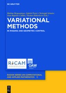
In the case of patch non-local means the error function in the functional is taken to be a g-weighted L2-norm. In the relaxed case with T > 0, we consider the case of fuzzy correspondences w(x, z),where z = (y, θ) ∈ Õ c×[0, 2π] stands for the center point y of patches outside the inpainting domain and their mutual rotation angle θ with respect to the patch around the center point x ∈ Õ in the (extended) inpainting domain.
We will consider the following variational framework for the functional ET, with a selectivity parameter T > 0: minimize

subject to

where

and H (w(x, ⋅, ⋅)) denotes the entropy of the probability distribution w(x, ⋅, ⋅)

We use the following notations: Ωp ⊂ ℝ2 is the patch domain, rθ : ℝ2 → ℝ2 is the rotation around the origin by an angle θ, that is in polar coordinates rθ(ρ, φ) = (ρ, φ+θ) and Rθ is the rotation operator acting on a function and rotating it by an angle θ around the origin, such that Rθ f(x) = f(rθ(x)) or equivalently, in polar coordinates Rθ f(ρ, φ) = f(ρ, φ + θ).We note that for f ∈ L∞ we have ‖f‖∞ = ‖Rθ f‖∞ and likewise for f ∈ BV, the space of functions of bounded variation: ‖f‖BV = ‖Rθ f‖BV, for any θ ∈ [0, 2π].
4.4.1.1Euler–Lagrange equations for ET
We recall the formulas for the solutions of the Euler–Lagrange equations for (4.1) which were derived in Section 4.3.1.2:
For a fixed u and minimizing with respect to w, we obtain the solution

where
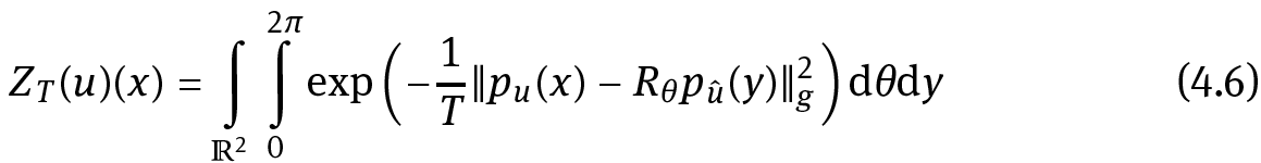
is the normalization to make w a probability density (to fulfill (4.2)).
When fixing w and optimizing with respect to u, the solution reads as

4.4.1.2Existence of minimizers of ET
In this section we will show the existence of minimizers of the energy functional in the case when the selectivity parameter T > 0. Throughout the whole section Lemma 4.4 will play a key role. To give sense to the rotations, we will only work in a two-dimensional setting. Similar results, without rotations, hold for the more general case in ℝd and we refer to [4] for a proof of convergence in this setting. The conceptual ideas for the proof of convergence in the rotation invariant setting go along the lines of [4], some results can even be used without further modification.
We assume Ω to be a rectangle in ℝ2, û ∈ L∞(Oc)∩BV(Oc) and u : Ω → ℝ such that u|Oc = û. In our energy functional (4.1) we implicitly understand that E T(u, w) = +∞ in case the integral in the second term is not defined. We also note that E T(u, w) is bounded below.
As admissible functions we define the set

where ? is given by

In this section we want to prove the existence of minimizers of the following problem

Clearly, in order to minimize ET the error between the two patches pu(x) and Rθpû (y) should be small whenever w(x, y, θ) is large. Unfortunately, the functional is not convex and consequently, the set of minimizers in ? must not be connected and non-optimal local minimizers might exist.
Proposition 4.1. Suppose  supp g ⊂ Ωp, and u ̂ ∈ BV(Oc) ∩ L∞(Oc).
Also let g be radially symmetric, that is g(h) = g(|h|). Then we have:
(i)If (un, wn) ∈ ? is a minimizing sequence for ET such that un is uniformly bounded, then it has a subsequence converging to a minimizer (u, w) ∈ ? of ET.
(ii)We can construct minimizing sequences as in (i), hence a minimizer (u, w) ∈ ? of ET exists. For any such minimizer we have u ∈ W1,∞(O) and w ∈ W1,∞(Õ × Õ c × [0, 2π]).
To prove the proposition we need the following two lemmas.
Lemma 4.2. Let A ∈ BV(ℝ2) and υ ∈ L∞(ℝ2), then constants C1, C2 > 0 exist such that the following estimates hold:

Proof. Let (ρε)ε be a family of mollifiers, which approximates the Dirac measure, and υε = υ ∗ ρε and Aε = A ∗ ρε. Then one can deduce from Hölder’s inequality that ‖υε‖∞ ≤ ‖υ‖∞ for any ε > 0. Furthermore, υε → υ in Lp for 1 ≤ p < ∞and υε converges weakly-* in L∞ to υ as ε → 0. Also, Aε → A in L1.
Clearly, for some ε > 0 any z ∈ ℝ2 we have that

for some C′ > 0. Since the statement holds for all z we deduce that

for some C1 > 0.
Let Fε(z) = ∫ℝ2 υε(h)Aε(h + z)dh and F(z) = ∫ℝ2 υ(h)A(h + z)dh. Then

Since A is an L1-function and υε converges weakly-* to υ in L∞ as ε → 0 the first term on the right-hand side tends to zero for ε → 0. For the second term on the right-hand side we have that

and as Aε → A in L1, we have that |F(z) − Fε(z)| goes to zero as ε → 0 for all z and hence F ε converges uniformly to F.
By (4.11), ‖∇Fε(z)‖∞ is bounded. By a Hölder estimate, also ‖Fε(z)‖∞ is bounded. Hence exists some function G(z) such that ∇Fε(z) converges weakly-* to G(z) in L∞. Let us now argue that G can be identified with ∇F in L∞. For ψ ∈ W1,1 we have that
where Dψ denotes the distributional derivative of ψ. Letting ε → 0 one obtains
and hence ∇F = G in the dual of W1,1. For any ϕ ∈ L1 there exists a sequence (ψε)ε, where ψε ∈ W1,1, and ψε → ϕ in L1 as ε → 0, which can for instance be obtained by convolution with suitable mollifiers. Hence, for ε → 0

and thus ∇F = G in (L1)′ = L∞ which implies that ∇Fε converges weakly-* to ∇F in L∞. By the Banach–Alaoglu theorem [1, Thm. 5.105] we have that

Combining (4.11) and (4.12) we have

which is the first estimate in (4.10).
The second estimate holds because

and hence C 2 > 0 exists such that

One repeats the argumentation from above to conclude the proof.
Remark 4.3. It is easily checked, that for the same constant C1 one can also obtain

since we take the L∞-norm over all z and the absolute value of the gradient remains unchanged.
Lemma 4.4. Let  supp g ⊂ Ωp, g radially symmetric, that is g(h) = g(|h|). Let û ∈ BV(Oc) ∩ L∞(Oc) and u ∈ L∞(Õ ), then the following functions are uniformly bounded in O × Õ c × [0, 2π].

Proof. First observe that the term can be split into three terms by evaluation of the squares:

The second term can be rewritten

Hence, the first two terms on the right-hand side of (4.14) are convolutions and we have the following estimates:

for ξ = x, y, θ.
Let us now examine the third term on the right-hand side of (4.14). In the case ξ = x, we have that

Choosing υ(h) = u(h) and A(h − x) = û(y + rθ(h − x))g(h − x), we can apply Lemma 4.2under consideration of Remark 4.3, since A is a BV-function with ‖A‖BV ≤ ‖û‖∞‖g‖BV + ‖g‖∞‖û‖BV [2, Remark 3.10]. We obtain that

By (4.15), (4.16), and (4.17), |∇x ∫ℝ2 (u(x+h)−û(y+rθ(h)))2g(h)dh| is uniformly bounded.
In the case ξ = y, we have that

Setting υ(h) = u(x + r−θ(h))g(h) and A(h + y) = û(h + y) we can apply Lemma 4.2 andobtain

Hence, |∇y ∫ℝ2 (u(x + h) − û(y + rθ(h)))2g(h)dh| is uniformly bounded.
In the case ξ = θ, we set υ(h) = u(x + h)g(h) and A(rθ(h)) = û(y + rθ(h)). Then the application of Lemma 4.2 yields

Since |∇θ ∫ℝ2 (u(x + h) − û(y + rθ(h)))2g(h)dh| is uniformly bounded by the estimates in (4.15), (4.16), and (4.19), we have concluded the proof.
We are now in a position to proof Proposition 4.1.
Proof of Proposition 4.1. We first prove (i). Let (un, wn) ∈ ? be a minimizing sequence for ET such that un is uniformly bounded.
If we define log+(t) := χ{t>1} log t, we observe that wn ↦ wn log+ wn is bounded in L1(Õ ×Õ c ×[0, 2π]) since the domain is bounded. Thus, we can say that wn is bounded in the Orlicz space L log+ L(Õ × Õ c × [0, 2π]). L log+ L can be seen as a function space which generalizes the usual Lp-spaces, instead of the convex function tp, 1 ≤ p < ∞, that characterizes the Lp spaces we consider the convex function t log+ t. A function f : X → ℝ is in L log+ L(X) if

As log+ t grows slower than any power function tr, r > 0, as t → ∞, for a bounded subset Ω ⊂ X we have that for ε > 0

and for 1 ≤ p < ∞

For more about Orlicz spaces we refer to [14] and [43].
Let us now argue that (wn)n∈ℕ is relatively weakly compact in L1. Since (wn)n∈ℕ is bounded and φ(t) = t log+ t is an increasing function satisfying (t log+ t)/t = log+ t → ∞as t →∞, we have that (wn)n∈ℕ is equi-integrable [2, Def. 1.26, Prop. 1.27]. Then we apply the Dunford–Pettis theorem to obtain that (wn)n∈ℕ is relatively weakly compact.
Since (wn)n∈ℕ is relatively weakly compact in L1 we may extract a subsequence (again called wn) which weakly converges to some w ∈ ?in L1(Õ × Õ c × [0, 2π]). By assumption, we know that un is uniformly bounded and hence exists a subsequence (again called un) which weakly converges to u in Lp, 1 < p < ∞, and weakly-* in L∞.
From Lemma 4.4 we know that the functions

are bounded by a constant depending on ‖un‖∞. However, since un is uniformly bounded the above gradients are bounded by a constant independent of n. Also ∫ℝ2 g(h)(un(x + h) − û(y + rθ(h)))2dh as a non-negative function of (x, y, θ) on a bounded domain has an upper bound that solely depends on ‖g‖1, ‖un‖∞ and ‖û‖∞ and therefore is bounded independently of n. Hence, we are in the position to apply the Ascoli–Arzelá theorem [48], which yields a subsequence, again denoted by unsuch that ∫ℝ2 g(h)(un(x + h) − û(y + rθ(h)))2dh converges uniformly and strongly in allLp spaces, 1 ≤ p ≤ ∞, as well as in the dual of L log+ L (see (4.21)) to some continuous function W(x, y, θ) as n →∞. Thus, we have that

We shall now demonstrate that ∫ w log w ≤ lim infn ∫ wn log wn. Since wn weakly converges to w in L1, by Mazur’s Lemma, see [23, Chap. 1], there exists a sequence of convex combinations w̄ n that strongly converges to w in L1. Then w̄ n → w almost everywhere and thus

Using the fact that t ↦ t log t is a convex function for t ≥ 0, we see that if (wn)n∈ℕ is such that ∫ wn log wn ≤ C, for some C > 0 and all n ∈ ℕthen also for the convex combinations w̄ n we have that ∫ w̄ n log w̄ n ≤ C and we can deduce that

such that (4.23) and (4.24) yield

Then, taking (4.22) and (4.25) together, we have shown that

We use the following estimate


Thus,

which proves (i) since (un, wn) is a minimizing sequence and (u, w) ∈ ?.
To prove the claim of (ii) let  be a minimizing sequence for ET. We define a sequence (un, wn) by

These are well defined and can be computed by the Euler–Lagrange equation, because the functional is bounded below and convex in one variable whenever the other variable is fixed. We observe that (un, wn) again is a minimizing sequence of ET since by (4.27) and (4.28) we have that

From the Euler–Lagrange equation with respect to u (4.7) and by Hölder’s inequality we see that ‖un‖L∞(O) ≤ ‖û‖∞, which allows us to apply (i), since we showed that un is uniformly bounded. Hence there is a minimizer (u, w) ∈ ? of ET.
We now want to show that u ∈ W1,∞(O) and w ∈ W1,∞(Õ ×Õ c×[0, 2π]) whenever (u, w) ∈ ? is a minimizer of ET.
First we want to show that the gradients ∇ξ, where ξ = x, y, θ, of w are bounded. For better readability we introduce  From Lemma 4.4 we know that ∇ξU(x, y, θ) are bounded for ξ = x, y, θ. Using (4.7) we again have that ‖u‖L∞(O) ≤ ‖û‖∞ and thus
is bounded below and above by positive constants, that is  Thus, we have that

are bounded. Since

is bounded we deduce that also

is bounded and hence w ∈ W1,∞(Õ × Õ c × [0, 2π]).
For x ∈ O we further have that

which is bounded by the argument above and therefore u ∈ W1,∞(O).
Remark 4.5. Note that whenever (u, w) ∈ ? fulfills (4.5) and (4.7), we have that u ∈ W1,∞(O) and w ∈ W1,∞(Õ × Õ c × [0, 2π]).
4.4.1.3Limit case T → 0
We are now interested in the case where the selectivity parameter T = 0. The idea behind this is that the fuzzy correspondence map w(x, y, θ) from the case T > 0 becomes a one-to-one correspondence map that determines the probability distribution. Clearly, these Dirac measures are no longer absolutely continuous with respect to the Lebesgue measure. We will therefore state some measure theoretic results which will be helpful for the remainder of this section. We will use the gained knowledge to propose a well-defined minimization problem for E 0, show the existence of minimizers, and examine their properties. As a last step we will show Γ-convergence of ET to E 0.
Now let ν be a positive Radon measure on ? × ?, such that ν(? × ?) = M < ∞and μ = π#ν the push-forward measure, see [2, Def. 1.70], where π : ? × ? → ? denotes projection on the first factor. Since  is a probability measure, the application of the disintegration theorem, see [2, Thm. 2.28], on the product space ? × ? and the projection π immediately yields the existence of a measurable measure-valuemap (in the sense of 2, Def. 2.25) x ↦ νx such that
  Then, by scaling back with factor M, the following statements about this measurable measure-value map x ↦ νx hold for arbitrary ψ ∈ L1(? × ?, ν):


For our application, we consider the case ? = Õ and ? = cl(Õ c)×[0, 2π] such that (y, θ) = z ∈ ? and ? is a subset of ℝ3.
Let us define the set ℳ to be the set of finite Radon measures ν ≥ 0 on ? × ? such that their restriction on the first component is equal to the Lebesgue measure on Õ , that is π#ν = ℒ2|Õ . Under the same assumptions on g and û as in Proposition 4.1 we further define
and for (u, ν) ∈ ?0

By the estimates on the integrand which were shown in Lemma 4.4, we derive that this integral is well defined for (u, ν) ∈ ?0.
We recall the solution to the Euler–Lagrange equation of E0(⋅, ν) for ν fixed, which was derived in (3.4) in Section 4.3.1.2:

Let us now discuss properties of the following minimization problem

We have the following theorem as a first result.
Theorem 4.6. Under the assumptions of Proposition 4.1 there exists a minimizer (u, ν) ∈ ?0 of E0.
Proof. Let (un, νn) ∈ ?0 be a minimizing sequence of E0. If un is not uniformly bounded, let ũ n := unχ|un|≤2‖û‖∞ be a truncated sequence constructed from un. Since for all x ∈ Õ and all y ∈ Õ c the following inequality holds
we deduce that

and hence (ũn, νn) is also a minimizing sequence. Thus, without loss of generality, we may assume un to be uniformly bounded and we can therefore extract a subsequence, again denoted by un, which weakly-*-converges to some u ∈ L∞(Ω) with u|Oc = û .From the proof of Proposition 4.1 we know that ∫ℝ2 g(h)(un(x + h) − û(y + rθ(h)))2dh converges uniformly to a continuous function W(x, y, θ). Conversely, wemay also assume that νn is relatively compact with respect to the weak-*-topology and thus admits a subsequence that weakly-*-converges to a measure ν [2, Thm. 1.59]. We will denote this subsequence again by νn. Some properties which hold for νn, n ∈ ℕ, are carried over to ν: From the weak-*-convergence, we have that
ν(V × cl(Õ c) × [0, 2π]) ≤ ℒ2(V), ∀V ⊂ Õ open ,
ν(K × cl(Õ c) × [0, 2π]) ≥ ℒ2(K), ∀K ⊂ Õ compact ,
and by the regularity of ν we obtain

Thus, we have that the projection π#ν = ℒ2|Õ and, as a consequence, ν ∈ ℳ.
Using the argument of (4.26), we have that

which yields

and therefore (u, ν) is a minimizer of E0.
Considering the case that φ: ? → ? is a measurable map, then, equivalently, x ↦ νx = δφ(x)(z) is measurable. In this way the measurable map φ determines a measure in ? that we will denote as νφ.
We will now state a result from [4], Prop. 3.
Proposition 4.7. There exists a minimizer (u∗, ν∗) ∈ ?0 of E0, such that ν∗ = νφ where φ: O ̃ → ? = cl(Õ c) × [0, 2π] is a measurable map.
For the proof, the interested reader is referred to [4]. One should read ? = Õ and ? = cl(Õ c) × [0, 2π] to make it work for the rotation invariant setting. Here we will just state the conceptual ideas: Berge’s maximum theorem [1, Thm. 17.31] applied to −U(x, z) = −∫ℝ2 g(h)(u(x + h) − û(y + rθ(h)))2dh, x ∈ ?, (y, θ) = z ∈ ?, yields that m(x) = minz∈Z U(x, z) is continuous and that the set-valued function M (x) = {z ∈ ?: U(x, z) = m(x)} is upper-hemicontinuous. Then by the closed graph theorem [1, Thm. 17.11] M (x) has a closed graph. The application of the Kuratowski–Ryll– Nardzewski theorem [1, Thm. 18.13] yields the existence of a measurable selector φ, such that E 0(u, νφ) = min(u,ν)∈A0 E 0(u, ν), which is the claim of the proposition.
As is further stated [4, Thm. 2], φ is not necessarily a BV-function. It only implies that for a given ε > 0exists Sε ∈ BV(?)m such that E0(u, νSε)≤ min(u,ν)∈A0 E0(u, ν)+ε. Because of this discrepancy, we will only be able to show convergence results for E 0 in the discrete setting (see Section 4.4.1.4).
With the proposition below we now address the interplay of the functionals ET and E 0.
Proposition 4.8. The energies ET Γ-converge to the energy E0 as T → 0 (in the sense of 2, Def. 6.12). In particular, the minimizers of ET converge to minimizers of E 0.
Proof. Let (un, wn) be a sequence in ? such that un weak-*-converges in L∞ to u and wn weak-*-converges as measures to ν, where (u, ν) ∈ ?0. Furthermore, let Tn > 0 be a sequence in ℝ such that Tn → 0. Since un weak-*-converges to u, exists N ∈ ℕ suchthat un is uniformly bounded for all n ≥ N. By Lemma 4.4, we have that ∫ℝ2 g(h)(un(x+h) − û(y + rθ(h)))2dh is uniformly Lipschitz for n ≥ N and converges uniformly to afunction W(x, z) = W(x, y, θ) and with ? = Õ c × [0, 2π], z = (y, θ) we have

Again, as we have seen in (4.26), we have that

and hence

Let us now show the lim sup-property. For (u, ν) ∈ ?0, let νx be the probability measure obtained by disintegrating ν with respect to ℒ2|Õ . We define un = u for all n and wn(x, z) = (mTn ∗ νx)(z), where mT(z) for T > 0 are a family of normed mollifier functions, which weak-*-converge as measures to the Dirac measure as T → 0. We have that wn ∈ ?, wn → ν weakly-* as measures, (un, wn) = (u, wn) ∈ ? for all n and

We have that

and therefore

Taking together the lim inf-property and the lim sup-property we have shown the Γ-convergence of ET to the energy E 0.
4.4.1.4Alternated optimization scheme
The algorithm used to minimize the energy describing the inpainting problemis based on an alternating optimization scheme.
4.4.1.4.1 T > 0
We will first consider the case T > 0.
Algorithm 4.9 (Alternated minimization of ET). Initialization: choose u0 with ‖u0‖∞ ≤ ‖û‖∞ For k ∈ ℕ solve

Under the assumptions made in Proposition 4.1 one may show the following result:
Proposition 4.10. The iterated optimization algorithm converges (modulo a subsequence) to a critical point of ET. The solution obtained (u∗, w∗) satisfies the regularity properties stated in Proposition 4.1, that is u∗ ∈ W1,∞(O) and w∗ ∈ W1,∞(Õ × Õ c × [0, 2π]).
Proof. Let h(u, w)(x, y, θ) = w(x, y, θ)(‖pu (x) −  + T log w(x, y, θ)), so that
 By the mean value theorem, and denoting z = (y, θ), we have that

for some w̃ (x, z) ∈ [wk(x, z), wk+1(x, z)]. From the equations (4.29), (4.30), and (4.31) in the proof of Proposition 4.1 we deduce that wk and wk+1 are bounded independentlyof k and, as a consequence, w ̃ is also bounded independently of k. Also, since wk+1 is the minimizer of E0(uk , w) with uk fixed, we have that  and, by direct computation,
  Hence exist C > 0 and γ > 0 such that

and thus

where the last inequality holds due to the minimality of uk+1 in E T(u, wk+1)when wk+1 is fixed. Summing up over all k = 0, . . . , N yields


By the equations (4.29), (4.30), and (4.31), we know that wk has a uniform Lipschitz bound. Hence, by the theorem of Ascoli–Arzelá, exists a subsequence wkj converging to some w∗ in Lp for 1 ≤ p ≤ ∞. Then, from (4.42) we have that also wkj+1 converges to w∗. Then by the Euler–Lagrange formula (4.7), we have that both ukj and ukj+1 converge to the same function u∗. If we let kj →∞in

and

we obtain the optimality conditions of u∗ and w∗ in the respective Euler–Lagrange equations (see (4.5) and (4.7)):