Piernicola Bettiol and Nathalie Khalil
9Non-degenerate forms of the generalized Euler–Lagrange condition for state-constrained optimal control problems
Piernicola Bettiol, Laboratoire de Mathématiques Unité CNRS UMR 6205, Université de Bretagne Occidentale, 6, Avenue Victor Le Gorgeu, 29200 Brest, France, [email protected]
Nathalie Khalil, Laboratoire de Mathématiques Unité CNRS UMR 6205, Université de Bretagne Occidentale, 6, Avenue Victor Le Gorgeu, 29200 Brest, France, [email protected]
Abstract: We establish nondegeneracy of the generalized Euler–Lagrange conditions for state-constrained optimal control problems, in which the dynamic is represented in terms of a differential inclusion depending on both time and state variables (allowing the case where the velocity set is just measurable w.r.t. the time variable), the state and the end-point constraints are closed sets. We propose here a new constraint qualification involving just tangent vectors to the state constraint (no inward pointing condition of the velocity set is required) and distance properties of trajectories to the end point constraints; this condition can be applied also when the minimizer has left end-point in a region where the state constraint set is nonsmooth. We finally provide an illustrative example.
Keywords: Optimal control, necessary conditions, differential inclusions, state constraints
AMS classification: 49J21, 49K21
9.1Introduction
Consider the state-constrained optimal control problem:

in which [S, T] is a given interval (S < T), g(., .) : ℝn × ℝn → ℝ is a given function, F (., .) : ℝ × ℝn ⇝ ℝn is a given multifunction with closed nonempty values, A, E0 and E1 are given closed nonempty subsets of ℝn. An absolutely continuous arc x(.) : [t1, t2] → ℝn ([t1, t2] ⊂ [S, T]) which satisfies the differential inclusion ẋ(t) ∈ F(t, x(t)), a.e. t ∈ [t1, t2], is called F-trajectory (on [t1, t2]). An F-trajectory x(.) for which the state constraint x(t) ∈ A is verified for all t ∈ [t1, t2] and the end-point constraint (x(S), x(T)) ∈ E0 × E1 is fulfilled, is called feasible.
We say that the feasible F-trajectory x̄(.) is a W1,1-localminimizer for (P), if there exists δ > 0 such that
for all feasible F-trajectories x(.) satisfying ‖x(.)− x̄(.)‖W1,1(S,T) ≤ δ. We shall also refer to x̄(.) as a W1,1 δ-local minimizer for (P) to better identify the positive number δ in the above definition.
First-order necessary conditions for optimality can be expressed in various forms (e.g., the generalized Euler–Lagrange conditions, the Maximum Principle), and play an important role in the selection and the characterization of solutions (minimizers) for problems in optimal control. When a state constraint appears in an optimal control problem, it may happen that, using the necessary conditions for optimality, the Lagrange multiplier associated with the objective function (to minimize) g(., .) takes the value zero (referred to as abnormal case). In this case, the objective function does not appear in the necessary conditions, and as a consequence it does not provide useful information to find the minimizers. A worse phenomenon, called also degenerate case, is well represented by classic examples (cf. [1] and [24]) which show that, in some circumstances, any feasible F-trajectory satisfies the necessary conditions, and therefore these give no information on the possible minimizers. Therefore, the nondegeneracy is a relevant issue in applying necessary optimality conditions. This explains the growing interest in the literature for nondegenerate forms (or even in the stronger version of normal forms) of necessary conditions for optimality (cf. [1, 14], [15, 16], and [21, 22], [5, 18], [17, 19], [8], and [4]). (We recall that “normal”means that the necessary conditions are valid with a nonzero Lagrange multiplier associated with the objective function.)
In this paper our main contribution is to establish nondegenerate forms of the generalized Euler–Lagrange conditions for optimal control problems as (P) above: the dynamic is represented in terms of a differential inclusion depending on both time and state variables, the state and the end-point constraints are just closed sets. We use an approach suggested in [21] and successively developed in earlier work: this requires exhibiting existence results of neighboring feasible trajectories (approximating a reference trajectory that possibly violates the state constraint) which allow one to obtain linear estimates w.r.t. the W1,1-norm. Known counter-examples (see [3] and [6]) highlight the fact that, in general, “classical” inward pointing conditions are not enough to derive linear W1,1-estimates for nonsmooth state constraints. However, recent papers [4] and [7] show that linear W1,1-estimates can still be considered for convex domains and Lipschitz continuous velocity sets satisfying a classical inward pointing condition if one of the following conditions occurs:
(i)the left end-point of the reference trajectory belongs to a region where the state constraint A is regular (i.e., the starting point is away from corners);
(ii)there is a complete freedom in the choice of the left end-point for the approximating trajectory;
(iii)the left end-point for the approximating trajectory can be chosen along hypertangent directions of the state constraint A.
(Observe that (ii) might actually be considered as a particular case of (iii).)
These neighboring feasible trajectories results were employed in [4] and [7] to prove normality of the generalized Euler–Lagrange conditions for free right end-point constraints (i.e., E1 = ℝn). In particular, condition (iii) is used to obtain normality when there exist hypertangent vectors in common between the state constraint A and the left end-point constraint E 0 (cf. [7]).
Here, we shall consider state-constrained differential inclusions which are just measurable with respect to the time variable, the state constraint is just a closed set (not necessarily locally smooth or convex), and we have both a left and a right end-point constraint. Nevertheless, employing some linear W1,1-estimates which turn out to be locally valid, we can still prove that the generalized Euler–Lagrange conditions for optimal control problems can be applied in the nondegenerate form (in the sense of (v) of Theorem 2.1 below) if one of the following constraint qualifications is satisfied:
(a)the left end-point of the reference minimizer x̄(.) belongs to a region where the state constraint A is regular (i.e., the starting point is away from corners), and a classical inward pointing condition is satisfied;
(b)there exist hypertangent vectors of the state constraint A; moreover, for all F-trajectories y(.) which are feasible on an initial (small enough) time interval and close to the reference minimizer x̄(.) (w.r.t. the W1,1-norm) the distance of the left end-point y(S) to E 0 ∩ A is strictly smaller than the distance of the right end-point y(T) to E1.
Thus, the novelties of this paper are the following:
–we allow the state constraint to be a closed set and the velocity set to be measurable w.r.t. the time variable, while in earlier work either some regularity assumption w.r.t. the time variable was imposed on the velocity set (for instance Lipschitz continuous cf. [1, 24]; or of bounded variation, see [20]), or the state constraint was represented by the intersection of regular sets, cf. [22];
–for the case in which a minimizer starts from a region where the state constraint is nonsmooth, we suggest a new constraint qualification in which no inward pointing condition involving the velocity set is required: the new condition invokes just hypertangent vectors of A and a property of F-trajectories close to the minimizer x̄(.) w.r.t. the W1,1-norm (see also (CQ b) of Theorem 2.1 below).
This paper is organized as follows. The main result (Theorem2.1) is stated in Section 2. Sections 3 and 4 are devoted to the proofs respectively of the main theorem and a crucial lemma on linear W1,1-estimates. The last section provides an example that illustrates the relevance of our new constraint qualification in proving the nondegeneracy of necessary optimality conditions.
Notation. We write ? the closed unit ball in Euclidean space, and | . | is the Euclidean norm. Given a nonempty set Y ⊂ ℝn, we write the interior, the convex hull and the closure of the convex hull of Y respectively int Y, co Y and  Y. The Euclidean distance of the point x from the set Y
  is written dY (x). Y∗ denotes the polar
cone of Y, namely
Given a closed nonempty set E ⊂ ℝn, we denote by πE(x) the set (possibly not a singleton) of the projections of the point x ∈ ℝn onto E, that is πE(x) := {y ∈ E : |y − x| =dE(x)}.
The limiting normal cone N E(x̄) of E at x ̄ ∈ E and the Clarke tangent cone TE(x̄) of E atx ̄ are defined as follows

and

The notation  means that xi → x ̄ and xi ∈ E for all i ∈ ℕ. We recall that the tangent cone TE(x̄) and the limiting normal cone N E(x̄) are related according to the following polarity relation
A vector ξ ∈ ℝn is called hypertangent vector of E at x ̄ ∈ E if and only if ξ ∈ int TE(x̄) (cf. [10]).
The graph, for a fixed t ∈ [S, T], of a multifunction F (t, .) : ℝn ⇝ℝn is the set
Consider a lower semi-continuous extended valued function f : ℝk → ℝ∪ {+∞} and a point x̄ ∈ dom f := {y ∈ ℝk : f(y) < +∞}.We recall that the limiting subdifferential ∂f(x̄) (sometimes also referred to as simply subdifferential) of f at x ̄ is defined to be

and can be expressed in terms of the limiting normal cone of the epigraph of f :
(For further details and discussion on these analytical tools we refer the reader to thebooks [2, 10] and [24] and the references therein.)
C ([t1, t2];ℝn) is the set of continuous ℝn valued functions on the time interval [t1, t2].We denote W1,1([t1, t2];ℝn) for the set of absolutely continuous ℝn valued functionson [t1, t2]; we shall employ the following norm on W1,1([t1, t2];ℝn):
which is equivalent to the classical W1,1-norm.
9.2Main result
We write A0 the set of all points y ∈ A where the state constraint A is locally regular: more precisely, y ∈ A0 if and only if there exists a radius r > 0 and a function h : ℝn → ℝ of class ?1+ (i.e., everywhere differentiable with locally Lipschitz continuous derivatives) such that

Observe that A0 ⊃ int A.
Theorem 2.1. Let x̄(.) be a W1,1 δ-local minimizer for problem (P), in which we assume that for some functions cF(.), kF(.) ∈ L1([S, T], ℝ+), the following hypotheses are satisfied:
(H1) The subsets A, E0, E1 ⊂ ℝn are closed.
(H2) (a) The multifunction F has nonempty, closed values, F (., x) is Lebesgue-measurable for each x ∈ ℝn;
(b)
(c)
(H3) g is Lipschitz continuous on (x̄(S) + δ?) × (x̄(T) + δ?).
(CQ) One of the following two conditions is satisfied:
(a)x̄(S) ∈ A0 and for some τ ∈ (0, T − S], c ≥ 1 and α > 0 we have ‖cF(.)‖L∞ ≤ c, and

(Here h(.) is the ?1+ function with the property in (2.1) for y = x̄(S).)
(b)int TA(x̄(S)) ≠ 0, and there exist numbers τ0 ∈ (0, T − S] and ρ0 ∈ (0, δ) such that for all arcs y(.) ≠ x̄(.) verifying the following inclusion
y(.) ∈ {x(.) ∈ W1,1([S, T], ℝn) : ẋ(t) ∈ F(t, x(t)) a.e. ,
‖x(.) − x̄(.)‖W1,1(S,T) ≤ ρ0 and x(t) ∈ A ∀ t ∈ [S, S + τ0]} ,
we have

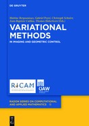
Then, there exist p(.) ∈ W1,1([S, T];ℝn), λ ≥ 0 and a function of bounded variation ν(.) : [S, T] → ℝn, continuous from the right on (S, T), such that
(i)for some positive Borel measure μ(.) on [S, T], whose support set satisfies
and some Borel measurable selection
we have
(ii)p(̇ t) ∈ co {η : (η, q(t)) ∈ NGr{F(t,.)}(x(̄t), ![]() t))} a.e. t ∈ [S, T] ,
t))} a.e. t ∈ [S, T] ,
(iii)(p(S), −q(T)) ∈ λ∂g(x̄(S), x̄(T)) + NE0∩A(x̄(S)) × NE1 (x̄(T)) ,
(iv)q(t) ⋅ x(t) =  q(t) ⋅ υ a.e. t ∈ [S, T] ,
(v)

in which q(.) : [S, T] → ℝn is the function

Remark 2.2. (a) We highlight the fact that the usual nonvanishing necessary condition (cf. condition (i) in [24, Theorem 10.3.1])

is here replaced by the nondegeneracy condition (v) in Theorem 2.1:

This constitutes a relevant aspect in applying necessary optimality conditions: consider, for instance, the case in which E0 = {x0} where x0 ∈ ∂A, then condition (2.2) does not allow one to consider trivial set of multipliers like
λ = 0, γ(.) = ξ, μ = δ{S}, p(.) ≡ −ξ ,
where ξ ∈ ![]() NA(x0) ∩ (? {0}) and δ{S} is the unit (Dirac) measure concentrated at {S}.
NA(x0) ∩ (? {0}) and δ{S} is the unit (Dirac) measure concentrated at {S}.
(b)If, under the assumptions of Theorem 2.1, we suppose in addition that F (., .) is convex valued, then (ii) implies also (cf. [24, Theorem 7.6.5])
(vi)p(̇ t) ∈ co {−ζ : (ζ, t)) ∈ ∂H(t, x̄(t), q(t))} a.e. t ∈ [S, T], where H is the Hamiltonian function:

9.3Proof of Theorem 2.1
We first observe that without loss of generality we may assume that the function c F(.) in (H2) is actually essentially bounded, also when we consider the case represented by condition (CQ b), replacing cF(.) with a constant c ≥ 1. This is standard reduction procedure based on a change of time variables (cf. [11]):

We state two lemmas, which have a key role in the proof of the nondegeneracy respectively in case (CQ a) and in case (CQ b) of Theorem 2.1.
Lemma 3.1 (Case where x̄(S) ∈ A0). Consider a (nonempty) closed set A ⊂ ℝn and a multifunction F : [S, T]×ℝn ⇝ℝn such that for some constants δ > 0, c ≥ 1, α > 0 and τ ∈ (0, T − S], for a function kF(.) ∈ L1([S, T], ℝ+), and for a given F-trajectory x̄(.), the assumptions (H2) and (CQa) of Theorem 2.1 are satisfied. Then, there exist constants ρ ∈ (0, δ), τ′ ∈ (0, τ] and K > 0 such that: given any F-trajectory x̂(.) on [S, T] and ε ≥ 0 satisfying

we can find an F-trajectory x(.) on [S, T] such that:

Lemma 3.1 represents a local version of known linear W1,1-estimates obtained for control systems with smooth state constraints (cf. [3]).
Lemma 3.2 (Case where x̄(S) ∈ A A0). Consider a (nonempty) closed set A ⊂ ℝn and a multifunction F : [S, T] ×ℝn ⇝ ℝn such that for some constants δ > 0, c ≥ 1, for a function kF(.) ∈ L1([S, T], ℝ+), and for a given F-trajectory x̄(.), the assumption (H2) of Theorem 2.1 is satisfied. Then, for any vector ῡ̄ ∈ int TA(x̄(S)), there exist constants ε̄ > 0, θ > 0, ρ ∈ (0, δ), τ ∈ (0, T − S] and K > 0 such that: given any F-trajectory x̂(.) on [S, T] and ε ∈ [0, ε̄] satisfying

and for any ẑ ∈ πA(x̂(S)), we can find an F-trajectory x(.) on [S, T] such that:

The proof of Lemma 3.2 will be provided in Section 9.4.
We shall continue the proof of Theorem 2.1 assuming that hypotheses (H1)–(H3) and (CQ b) are satisfied. For the case in which hypothesis (CQ a) is assumed [instead of (CQ b)], the theorem can be proved applying a similar technique (invoking Lemma 3.1 instead of Lemma 3.2), cf. also the proof of [22, Theorem 2.1].
The proof approach is along similar lines to that of [22]. Nevertheless, since the nature of the state constraints (and in turn the related distance estimates provided by Lemma 3.2) differs from that of [22], the analysis employed herein requires some ideas that are new with respect to the earlier work.
To begin with, assumption (CQ b) of Theorem 2.1 guarantees the existence of a vector ῡ̄ ∈ int TA(x̄(S)), which means that all the assumptions of Lemma 3.2 are satisfied.
Consider the constants ε̄ > 0, θ > 0, ρ ∈ (0, δ), τ ∈ (0, T − S], and K > 0 provided by Lemma 3.2. We can always suppose also that τ ≤ τ0 and ρ ≤ ρ0 [where τ0 and ρ0 are the constant given by condition (CQ b)]. Take any arbitrary sequence εi ↓ 0 with εi ≤ ε̄ and, for each i ∈ ℕ, set the function ϕi : ℝn × ℝn × ℝ+ → ℝ:
Define also the sets of functions
X := {y(.) ∈ W1,1([S, T], ℝn ) : ẏ(t) ∈ F(t, y(t)) a.e. and
‖y(.) − x̄(.)‖W1,1(S,T) ≤ ρ} ,
Consider now the space X with the metric induced by the W1,1-norm. Then, X turns out to be complete. Notice also that (w.r.t. the topology induced by the W1,1-norm) the set X1 is closed. Moreover, the function Φi : X →ℝ

is continuous on X, and so it is continuous also on X1. Since x̄ (.) ∈ X1 is an  minimizer for Φi on X 1, for each i ∈ ℕ, Ekeland’s Theorem (cf. [24, Theorem 3.3.1]) guarantees the existence of an arc xi(.) ∈ X1 such that
and such that the functional
attains a (unique) minimum at xi(.). As a consequence, by eventually a subsequence extraction, we obtain that

By extracting subsequences (without relabeling) we can arrange that either of the following situations arises:
(a)xi(.) ≠ x̄(.), for all i = 1, 2, 3, . . . or
(b)xi(.) ≡ x̄(.), for all i = 1, 2, 3, . . . .
Notice also that the functional Ji(.) is, in fact, uniformly Lipschitz continuous on X with respect to the W1,1-norm. Let KJ > 0 be a constant independent of i such that

Associated with any minimizer xi(.) for Ji(.), we define the positive number

The following lemma is an easy consequence of the Max-rule for subdifferentials, and the fact that either xi(.) ≠ x̄(.) or xi(.) ≡ x̄(.) for all i = 1, 2, 3, . . . . Observe that, in the first case, owing to assumption (CQ b), since each xi(.) ∈ X1, we have that dE0∩A(xi(S)) < dE1 (xi(T)).
Lemma 3.3. Take any subgradient
where xi(.)’s are the minimizers for Ji(.) and di’s are the corresponding numbers defined in (3.5). Then for all i large enough, we obtain either
for some a ≥ 0 and ξ1 ∈ NE1 (e1), in which e1 ∈ πE1 (xi(T)) and
or
(b)(xi(.) ≡ x̄(.))
Lemma 3.4. Assume that the hypotheses of Lemma 3.2 hold true. Then there exists i0 ∈ ℕ such that, for all i ≥ i0, xi(.) is a W1,1-local minimizer for the problem

Proof. The proof of this lemma is based on a standard penalization argument, which is applicable owing to Lemma 3.2. Wewrite the proof here in detail to highlight the role of the W1,1-linear estimate provided by Lemma 3.2. Since εi ↓ 0 with εi ≤ ε̄, there exists i0 ∈ ℕsuch that we also have  for all i ≥ i0. Suppose, for contradiction, that the statement is false. Recall that ῡ̄ ∈ int TA(x̄(S)) is given by assumption (CQ b). It follows that we can choose
  such that for all j ∈ ℕ, j ≥ i0, there exist i ≥ j and ŷ(.) ∈ X such that
and
Write  Observe that
  and the fact that thexi(.)s belong to X1, guarantees that ε ≤ δ′ ≤ ε̄. Then, owing to Lemma 3.2 (applied for the F-trajectory ŷ(.) and for the violation of the state constraint on [S, S + τ]), there exist θ > 0 and an F-trajectory y(.) on [S, T] such that

Bearing in mind that also

(for x̄(.) is feasible), it follows that
and therefore y(.) ∈ X1. Moreover, we would have

which contradicts the minimality of xi(.) on X1.
A consequence of Lemma 3.4 is that, for i ∈ ℕ with i ≥ i0, the state trajectory

is a W1,1-local minimizer for the state-constrained optimal control problem

in which the (final) cost is

the velocity set is represented by the multivalued function
and the function h̃ : [S, T] × ℝn × ℝ× ℝ × ℝ → ℝ (which provides the state constraint by means of a functional inequality) is defined by:

Assume now that we are in case (a): xi(.) ≠ x̄(.), for all i.
Notice that the necessary conditions for the optimality referred to problem (3.7) [24, Theorem 10.3.1] are applicable, and, consequently, for each i, we obtain a constant λ̃i ≥ 0, a function p̃i(.) = (pi(.), χi(.), ζi(.), ψi(.)) ∈ W1,1([S, T];ℝn+3), which is the costate trajectory associated with the state x̃i(.), a Borel measurable function μi(.) on [S, T] and a μi-integrable function γ̃i : [S, T] → ℝn+3, such that
(i)′ ‖p̃i‖L∞(S,T) + λ̃i + ∫[S,T] dμi(s) = 1 ,
(ii)′ pi(t) ∈ co { η ̃∈ ℝn+3 : ( η, ̃ qĩ (t)) ∈ NGr{G(t,.)}( xĩ (t), xi (t))} a.e. t ∈ [S, T] ,
(iii)′(p̃i(S), −q̃i (T)) ∈ λ̃i∂g̃(x̃i(S), x̃i(T)) + 
(iv)′ q̃ i(t) ⋅ t) =  a.e. t ∈ [S, T] ,
(v)′  and supp{μi} ⊂ {t : h̃(t, x̃i (t)) = 0}
in which q̃i(.) : [S, T] → ℝn+3 is the function

supp μi denotes the support of the measure μi, and  is the set
![]() h̃(t, x̃) := co { ζ : there exist x̃j → x̃, tj → t and ζj → ζ s. t.
h̃(t, x̃) := co { ζ : there exist x̃j → x̃, tj → t and ζj → ζ s. t.
We observe that the Euler–Lagrange inclusion (ii)′, the transversality condition (iii)′ and condition (v)′, bearing in mind the information provided by Lemma 3.3, imply that there exist (for i large enough)  such that (vi)′
 , and
, and  , (vii)′
 , where
and

Since the multivalued map G is kF(.)-Lipschitz w.r.t. the state variable around the G-trajectory x̃(.) (recall that, around the reference F-trajectory x̄(.), kF(.) is the function as defined in Theorem 2.1), we notice that (ii)′ implies also that

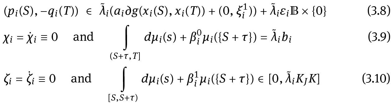
Notice that the necessary conditions apply in the normal form. Indeed, assume that λ̃i = 0, then from (3.8)–(3.11), we would obtain

which, combined with (3.13), would imply p̃i ≡ 0 (using Gronwall’s Lemma). But this contradicts (i)′.
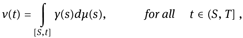
The above relations are valid for arbitrary i ∈ ℕ sufficiently large. Standard convergence analysis (cf. [22] or [24]), following the extraction of subsequences, providesthat  for some constants λ̃ ≥ 0 and a, b, β0, β1 ∈[0, 1],
  → ξ1 ∈ ℝn for some vector ξ1 ∈ ℝn ∩ ?. Furthermore, pi(.) → p(.) uniformly, pi(.) → ṗ(.) weakly in L1, μi(.) → μ(.) and γi(.)μi(.) → γ̄(.)μ(.) in the appropriate weak-* topology (where γi(.), having its values in ℝn, is relative to the adjointarc pi(.) and it represents the first component of γ̃i(.)) and qi(.) → q(.) a.e., for someabsolutely continuous function p(.), function of bounded variation q(.), Borel measure μ(.) and μ-integrable function γ̄(.). The limit of the relationships (i)′, (iv)′-(vii)′,(3.8)–(3.12) yield
(i)″ ‖p‖L∞ + 2λ̃ + ∫[S,T] dμ(s) = 1 ,
(ii)″ p(̇ t) ∈ co {η ∈ ℝn : (η, q(t)) ∈ NGr{F(t,.)}( x(̄ t), x(t))} a.e. t ∈ [S, T] ,
(iii)″(p(S), −q(T)) ∈ aλ̃∂g(x̄(S), x̄(T)) + λ̃(0, ξ1) ,
(iv)″q(t) ⋅ x(t) =  q(t) ⋅ υ a.e. t ∈ [S, T] ,
( v)″∫(S+τ,T] dμ(s) + β0μ({S + τ}) = λ̃b and ∫[S,S+τ) dμ(s) + β1μ({S + τ}) ∈ [0, λ̃KJK] ,
(vi)″a + b + |ξ1| = 1, and β0 + β1 = 1 ,
(vii)″ξ1 ∈ NE1 (x̄(T)) ∩ ?
in which q(.) : [S, T] → ℝn is the function

where γ(.) := (γ̄(.))p, that is the first n-components of the μ-integrable function γ(.), corresponding to the p-variable. The state constraint in the optimal control problem (3.7) is formulated as a functional inequality constraint by means of the function h̃ ,which in turn involves the distance function to the set A, dA(.). This translates into necessary optimality conditions for our reference problem (P), in which we assume implicit state constraints (i.e., the state constraint set is a general closed set). The simple analysis, involved in deriving the necessary conditions for the implicit constraints from the necessary conditions for the functional inequality constraints, is described in [24] (see Remark (e) p. 332, and Remark (b) p. 370). This allows us to obtain property (i) of Theorem 2.1.
Observe that using the same argument as for the multipliers λ̃i, we conclude that λ̃ ≠ 0. Define λ := aλ̃. Then, λ, p(.), ν(.) := ∫[S,.] γ(s) dμ(s) satisfy assertions (ii)–(iv) of the theorem statement.
It remains to prove the nondegeneracy condition (assertion (v) in the statement of Theorem 2.1):

Assume to the contrary that (3.14) is violated. Then λ = 0 (which, since λ̃ ≠ 0, implies a = 0), |p(S) + ν({S})| = 0 and ∫(S,T] dμ(s) = 0, that together with the first condition of (v)″ gives b = 0. As a consequence, from the first equality in (vi)″ we obtain that |ξ1| = 1, and therefore, owing to (iii)″,

Conversely, invoking Gronwall’s inequality, conditions ∫(S,T]dμ(s) and |p(S) + ν({S})| above yield:

The two relations (3.15) and (3.16) provide a contradiction. Thus, we have proved also the nondegeneracy condition (3.14).
Assume finally that we are in case (b): xi(.) ≡ x̄(.), for all i.
Necessary optimality conditions for problem (3.7) still apply, providing the same conditions (i)″–(v)″ and (vii)″ above, whereas (vi)″ is replaced by:
(vi)″a = 1, and β0 + β1 = 1 .
This immediately implies that the Lagrange multiplier associated with the cost function λ = λ̃ > 0, and therefore, in this case the necessary conditions are nondegenerate (in fact they apply in the normal form), and this concludes the proof of Theorem 2.1.
9.4Proof of Lemma 3.2
Fix any ῡ̄ ∈ int TA(x̄(S)). Invoking the characterization of the interior of the Clarketangent cone, we can find  such that

Define  and
and  such that
  Define also
  Consider any F-trajectory x̂(.) and any ε ∈ [0, ε̄] for whichcondition (3.2) is valid.
Fix now by ẑ0 any element in πA(x̂(S)). Condition (3.2) clearly ensures that |ẑ0 − x̂(S)| ≤ ε . Invoking the Filippov Existence Theorem (cf. [2] or [24]) to the reference trajectory x̂(.), we obtain an F-trajectory ẑ(.) on [S, T] such that:

Notice that:

Write  Notice that since
 Define the arc z(.) as follows:
Since  dA(ẑ(t)) ≤ ε′, for all t ∈ [S, S + τ], we have

Take any y ∈ πA(ẑ(t)), then we can easily establish the following estimate for all t ∈ (S, S + τ]:

It follows that from the choice of δ0, ρ and τ, we have ∀t ∈ [S, S + τ]:

Consequently, (4.1), (4.2) and (4.3) ensure that

We apply once again the Filippov Existence Theorem considering ẑ(.) as a reference arc and z(S) = ẑ(S) + θ0ε′ῡ̄ as the new initial state point [recall that ẑ(S) = ẑ0 ∈ πA(x̂(S))]: we obtain an F-trajectory x(.) such that x(S) = z(S) and for all t ∈ (S, T]:

Therefore, since x(S) = z(S) and ż (t) = z(t) a.e., we have

Then, from the choice of τ,

We deduce from the relations (4.4) and (4.6) above that x(t) ∈ z(t) + ε′? ⊂ A, ∀t ∈ [S, S + τ] . Furthermore, invoking again (4.5), we have:

Finally, notice that:

The validity of (3.3) follows taking the constant  in the expressionof x(S) and
  for the desired linear W1,1-estimate.
9.5Example
We provide an example to illustrate the result provided by Theorem 2.1, when the left end-point of the minimizer belongs to a region in which the state constraint is non-smooth. The example illustrates the relevance of the constraint qualification (CQ b): this implies the nondegeneracy of the necessary optimality conditions even if a (convexified) inward pointing condition (for the velocity set) is not necessarily satisfied. In this example we have a discontinuous time-dependent velocity set.
Example. We consider the optimal control problem with state constraints:

where

in which  for k = 0, 1, 2, 3, . . .
Consider the arc z(.) : [0, 1] → ℝ defined as: z(0) = 0, z(tk ) := (−1)k tk, and ż(t) = (−1)k2 for t ∈ (tk+1, tk], Then, the F-trajectory
is a W1,1 minimizer for problem (P1), for x̄(0) = (0, 0, 0) ∈ E0, x̄(1) = (1, 1, 0) ∈ E1 and x̄3(1) = 0.We claim that condition (CQb) is satisfied. Indeed, clearly int TA(x̄(0)) ≠ 0. Fix now any τ0 ∈ (0, 1) and ρ0 > 0. Consider the family of F-trajectories
X1 := {x(.) ∈ W1,1([0, 1], ℝ3) : ẋ(t) ∈ F(t) a.e. ,
‖x(.) − x̄(.)‖W1,1(0,1) ≤ ρ0 and x(t) ∈ A ∀ t ∈ [0, τ0]} .
Observe that for all y(.) ∈ X1 such that y(.) ≠ x̄(.), we necessarily have y(0) = (y1(0), y2(0), y3(0)) ∈ A and, so, y1(0) > 0.
Moreover, if y3(1) = 0, then it follows that y(1) = y(0) + x̄(1), and we immediately have
If y3(1) > 0, then we obtain

We have proved the claim.
Therefore, the necessary conditions apply in the nondegenerate form (in the senseof (v) of Theorem 2.1).
Conversely, if we had a different choice for the left end-point condition in problem (P1), for instance E0 = {(0, 0, 0)} (observe that in this case (CQ b) is not verified), then the necessary conditions for optimality would be compatible with the degeneracy condition

Indeed, it is easy to verify that the necessary conditions of optimality to the reference minimizer x̄(.), would be applicable in a degenerate form provided that (p(.) ≡ const)

and

Notice that (5.2) is just the left end-point transversality condition, whereas (5.3) follows immediately from the degenerate condition (5.1) and from the fact that ν({0}) ∈ N A(x̄(0)). As a consequence, the (standard) necessary conditions apply (in the degenerate form) not only for the minimizer x̄(.) but also for any feasible F-trajectory x(.) having x(0) = (0, 0, 0) as left end-point. This is possible with the trivial choice of multipliers λ = 0, γ = ξ, μ = δ{0}, p(.) = −ξ, in which ξ ∈ NA((0, 0, 0)) ∩ (? {0}) and δ{0} is the unit measure concentrated at {0}.
Bibliography
[1]A. V. Arutyunov and S. M. Aseev, Investigation of the degeneracy phenomenon of the maximum principle for optimal control problems with state constraints, SIAM J. Control Optim., 35:930–952, 1997.
[2]J. P. Aubin and H. Frankowska, Set-valued Analysis. Birkhäuser, Boston, 1990.
[3]P. Bettiol, A. Bressan, and R. B. Vinter, On trajectories satisfying a state constraint: W1,1 estimates and counter-examples. SIAM J. Control Optim., 48:4664–4679, 2010.
[4] P. Bettiol and G. Facchi, Linear estimates for trajectories of state-constrained differential inclusions and normality conditions in optimal control, J. Math. Anal. Appl., 414:914–933, 2014.
[5]P. Bettiol and H. Frankowska, Normality of the maximum principle for non convex constrained Bolza problems, J. of Differential Equations, 243 (2007), no 2, 256–269.
[6]P. Bettiol, H. Frankowska, and R. B. Vinter, L∞ estimates on trajectories confined to a closed subset, J. of Differential Equations, 252:1912–1933, 2012.
[7]P. Bettiol, N. Khalil, and R. B. Vinter, Normality of generalized Euler–Lagrange conditions for state constrained optimal control problems, J. Convex Anal., 23(1):291–311, 2016.
[8]P. Bettiol and R. B. Vinter, Trajectories Satisfying a Smooth State Constraint: Improved Estimates, IEEE TAC, 56(5):1090–1096, 2011.
[9]A. Bressan and G. Facchi, Trajectories of differential inclusions with state constraints. J. Differential Equations, 250:2267–2281, 2011.
[10]F. H. Clarke, Optimization and Nonsmooth Analysis, Wiley-Interscience, New York, 1983.
[11]F. H. Clarke, Necessary Conditions in Dynamic Optimization, Memoirs of the American Mathematical Society, no. 173, 2005.
[12]A. Yu. Dubovitskii, A. A. Milyutin, Extremum problems with constraints, Soviet Math., 4:452– 455, 1963.
[13]A. Yu. Dubovitskii, A. A. Milyutin, Extremum problems in the presence of restrictions, U.S.S.R. Comput. Math. Math. Phys., 5(3):1–80, 1965.
[14]M. M. A. Ferreira, F. A. C. C. Fontes, and R. Vinter, Nondegenerate necessary conditions for non-convex optimal control problems with state constraints, J. Math. Anal. Appl., 233(1):116–129,1999.
[15]M. M. A. Ferreira and R. Vinter, When is the maximum principle for state constrained problems nondegenerate?, J. Math. Anal. Appl., 187(2):438–467, 1994.
[16]F. A. C. C. Fontes, S. O. Lopes, and R. de Pinho, On constraint qualifications for nondegenerate neccesary conditions of optimality applied to optimal control problems, Discrete Contin. Dyn. Syst., 29(2):559–575, 2011.
[17]F. A. C. C. Fontes and S. O. Lopes, Normal forms of necessary conditions for dynamic optimization problems with pathwise inequality constraints, J. Math. Anal. Appl., 399(1):27–37, 2013.
[18]H. Frankowska, Normality of the maximum principle for absolutely continuous solutions to Bolza problems under state constraints. Control Cybernet., 38(4B) (2009), 1327–1340.
[19]H. Frankowska and D. Tonon, Inward Pointing Trajectories, Normality of the maximum principle and the non occurrence of the Lavrentieff phenomenon in optimal control under StateConstraints, J. Convex Anal., 20(4):1147–1180, 2013.
[20]M. Palladino and R. B. Vinter, Regularity of the Hamiltonian along Optimal Trajectories, SIAM J. Control Optim., 53:1892–1919, 2015.
[21]F. Rampazzo and R. B. Vinter, A theorem on existence of neighboring trajectories satisfying a state constraint, with applications to optimal control. IMA J. Math. Control Inform., 16:335–351, 1999.
[22]F. Rampazzo and R. B. Vinter, Degenerate optimal control problems with state constraints. SIAM J. Control Optim., 39:989–1007, 2000.
[23]R. T. Rockafellar, Clarke’s tangent cones and the boundaries of closed sets in ℝn, Nonlinear Anal., 3(1):145–154, 1979.
[24]R. B. Vinter, Optimal Control, Birkhäuser, Boston, 2000.