Hint. Apply the twisted conjugacy theorem to each H (R + ⋅, ⋅), with R ∈ ℝn close to 0 such that the torus r = R is Diophantine for Ko and, using Proposition 4.4, extend the so-obtained function R ↦ β(R) as a smooth function.
Bibliographical comments.
–It is possible to give a proof, patterned on [87, p. 626], that ψ is C1 without the assumption that ϕ′(x) has unique inverse (or right inverse). Yet the proof simplifies and the estimates improve under the combined two additional assumptions. In particular, the existence of a right inverse of ϕ′(x) makes the inverse ψ unique and, thus, allows us to ignore the way it was built (a posteriori regularity result).
–Latzutkin understood, in the case of the standard map, the fundamental importance of Whitney-smoothness of the invariant circles with respect to the rotation number. This is a key point in the method of parameter. The dependance actually is of Gevrey class [77], but we do not need it here.
13.5Conditional conjugacy
We now move to a conditional conjugacy, the common ground of invariant tori theorems of later sections.
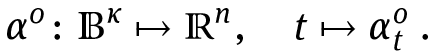
Let
be the set of Hamiltonians on  for which T0 is invariant and quasiperiodic, with unprescribed frequency.
Theorem 5.1 (Conditional conjugacy). For every Ko ∈ ?s+σ(αo), with αo ∈ Dγ,τ, there is a germ of smooth map28
at Ko ↦ (Ko, id) such that the following implication holds:
and (KH, GH) is unique in ? × ?.
Proof. Denote ϕα the operator we have been denoting ϕ because the frequency α wasfixed while we now want to vary it. Define the map

locally in the neighborhood of (αo , Ko). Since ϕ is infinitely differentiable, by Proposition 4.4, there exists a C∞-extension
Write Ko = αo ⋅ r + K̂ , K ̂ = c + O(r2). In particular, since
locally for all α ∈ ℝn close to αo, we have
In particular,

and, by the implicit function theorem, locally for all H, there exists a unique α̂ such that β(α̂, H) = 0.We conclude by letting Θ(H) = Θ̂ (α̂, H).
The so-defined vector αH, which is called a frequency vector of H, is unique when belonging to Dγ,τ. It depends Gevrey-smoothly on H (i.e., their partial derivatives of order r behave like positive powers of r!), as discovered by Popov [77], but not analytically (except for a family of integrable Hamiltonians). (For our purpose, the Lipschitz regularity would suffice, in conjunction with the Lipschitz inverse function theorem. For the sake of simplicity, we stick to the C1 class.)
13.6Invariant torus with prescribed frequency
The first invariant torus theorem will be a trivial corollary of the conditional conjugacytheorem. Consider a smooth family  of Hamiltonians in some ?s. Each
  isof the form The frequency map of the family is

In this section, we will describe the simplest case, where (the derivative of) αo has rank n, which, by the submersion theorem, implies that αo is onto, stably with respect to C1-perturbations. In celestial mechanics, the parameter t may be masses, semimajor axes, eccentricities, inclinations, energy, angular momentum, etc.
Now, let (Ht) be a smooth family of Hamiltonians in ℋs such that, for each t, Ht is close enough to Kt (a condition that we will not repeat in each statement).
Theorem 6.1. If the frequency map αo is a local submersion (i.e., of rank n) and if αo(0) ∈ Dγ,τ, there exists t ∈ ?n such that Ht has an invariant torus with frequency αo(0).Moreover, the subset formed by the values of t ∈ ?n for which Ht has an invariant torus has positive Lebesgue measure.
Proof. According to the conditional conjugacy theorem, the family (Ht) has some frequencymap α which is C∞-close to αo. So α itself is a local C∞-submersion and attains αo(0). Besides, as soon as αt ∈ Dγ,τ, Ht has an invariant torus, which occurs for a subset ℬ ⊂ ?n of positive Lebesgue measure.
Remark 6.2. The first part of the conclusion holds under the topological hypothesis that αo has nonzero degree (which ensures that αo is locally onto, stably with respect to perturbations), a remark which applies if αo has a ramification point, for example.
Poincaré [76] introduced the following two transversality conditions (he was considering the particular case, considered next, where t is the action variable, Ko = Ko(r) and α = ∂rKo(r)).
Definition 6.3. The Hamiltonian family  is
is
–isochronically nondegenerate if the frequency map has rank n
–isoenergetically nondegenerate if the map

(where  stands for the homogeneous class of α) has rank n. (Neither condition implies the other.)
Exercise 6.4 (Variants of Theorem 6.1). Prove the following two variants.
–Isoenergetic theorem: If the family (Kt) is isoenergetically nondegenerate, and if the frequency vector αo belongs to Dγ,τ, there exists t ∈ ?κ such that Ht has aninvariant torus of energy ![]() and frequency class
and frequency class  Moreover, the subset formedby the values of t ∈ ?κ for which Ht has an invariant torus of energy
 ![]() has a positive (n − 1)-dimensional Lebesgue measure.29
has a positive (n − 1)-dimensional Lebesgue measure.29
–“Iso first integral” theorem: More generally, assume that for all t, ft is an ℝλ-valued first integral of  and Ht (e.g., with λ = 2, ft may stand for the energy and the angular momentum of a mechanical system in the plane) and that the frequency vector αo belongs to Dγ,τ The function ft must be constant on T0 and we call ft(T0) this constant. If the map

has the maximal rank n, there exists t ∈ ?κ such that Ht has an invariant torus on which ft = f0(T0) and with the frequency class  More strongly, if the map

has the maximal rank n, for every to ∈ ?κ close to 0, there exists t ∈ ?κ such that Ht has an invariant torus with ft = f0(T0) and frequency vector 
(For a first integral associated with a non-Abelian symmetry, see Section 13.8.)
We now turn to Kolmogorov’s theoremwhich corresponds to the particular case where the family (Ht) is obtained by mere translation of some initial Hamiltonian H ∈ ℋ, in the direction of actions: Ht(θ, r) = H(θ, t + r), t ∈ ?n. Call co and Qo the constant and quadratic parts of some Ko ∈ ?(αo), respectively:
Theorem 6.5 (Kolmogorov). If the frequency vector αo belongs to Dγ,τ and if the quadratic form ∫?�n Qo(θ) dθ is nondegenerate, there exists a unique R ∈ ℝn such that G−1(T0)+ (0, R) is an αo-quasiperiodic invariant torus of H. Moreover, the invariant tori of H form a set of positive Lebesgue measure in the phase space.
Proof. Let F be the analytic function taking values among symmetric bilinear forms, which solves the cohomological equation  (use Lemma (B.1)), and ψ be the germ along T0 of the (well-defined) time-onemapof the flow of the Hamiltonian F (θ) ⋅ r2. The map ψ is symplectic and restricts us to the identity on T0. At the expense of substituting Ko ∘ ψ and H ∘ ψ for Ko and H, respectively, one can thus assume that

The germs so obtained from the initial Ko and H are close to one another.
Consider the family of trivial perturbations obtained by translating K o in the direction of actions:

and its approximation obtained Roby truncating the first-order jet of  along T0 from its terms O(R2):

For the Hamiltonian  T0 is invariant and quasiperiodic of frequency αo + 2Q1 ⋅ R.The first assertion then follows from Theorem 6.1.
What has been done for the torus of frequency αo can more generally be done for all tori of Diophantine frequency. What remains to be proved is that the collection of perturbed invariant tori has a positive measure. Using the map Θ of the conditional conjugacy theorem, we now define
with

locally in the neighborhood of R = 0, say for ‖R‖ < R0.Let
As soon as  is invariant for HR,

is invariant for H. Because of Proposition 4.4, ?R depends Whitney-smoothly on R ∈ ℛ. Thus, the diffeomorphisms which straighten all the ?R’s individually may be glued together, by Whitney’s extension theorem and the last assertion follows.
Remark 6.6 (Measure of the set of tori). Due to the estimate of the inverse function Theorem 3.1, if γ ≪ 1, the allowed size of |H−Ko|s (for some s > 0) is polynomial in γ (of degree 4). One can actually show that it is |H − Ko|s = O(γ2) [78]. In other words, for a given H, a torus with frequency vector in Dγ,τ is preserved for some  and, as a classical estimate of the measure of the complement of Diophantine vectors shows, the measure of the complement of the invariant tori is of the order
Once one has one invariant torus, it is straightforward to obtain a set of positive measure of invariant tori, as the proof above has shown. (This was not so at the level of generality of Theorem 6.1. Why? If t1, t2 ∈ ℬ, the invariant tori of Ht1 and Ht2 may meet. In Kolmogorov’s theorem, the parameter being the cohomology class of the tori, this cannot happen.) We will see in the next section that a much weaker transversality condition is sufficient for locally finding a positive measure of tori. Yet, in the absence of any transversality hypothesis, the question of the accumulation of a quasiperiodic invariant torus by quasiperiodic invariant tori, and their measure, is the subject of Herman’s conjecture [33].
Exercise 6.7. Instead of applying Theorem 6.1, complete the proof of Theorem 6.5 using the twisted conjugacy theorem.
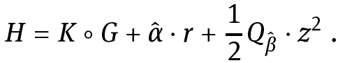
Hint. The twisted conjugacy normal form of  with respect to the frequency α is

By assumption, the matrix  is invertible and the map
  is a localdiffeomorphism. Now, there is an analogous map R → βR for HR, which is a small C∞-perturbation of
  and thus a local diffeomorphism, with a domain having a lower bound locally uniform with respect to H. Hence, if H is close enough to Ko, there is a unique small R such that β = 0. For this R, the equality HR = K ∘ G holds; hence, the torus obtained by translating G−1(T0) by R in the direction of actions is invariant and α-quasiperiodic for H.
Bibliographical comments.
–Claims that Kolmogorov’s proof was incomplete are unfounded in view of the breakthrough: the supposedly missing arguments in Kolmogorov’s paper bear upon to Cauchy’s inequality and elementary harmonic analysis [22, 39, 56]. Kolmogorov actually gave these details in Moscow’s seminar, as Arnold and Sinaï have testified. Arnold later gave an alternative proof. Arnold’s statement is equivalent to Kolmogorov’s statement, despite the superficial difference of looking to all neighboring tori at a time. Arnold additionally paid attention to how far H can be from Ko, as the torsion gets close to degenerate [2].
–The remark that parameters are not necessarily action variables adds some flexibility for finding invariant tori, for example, in the work of Zhao [103, 104]. Another example is an analog of Arnold’s theorem where one would be allowed to tune not only the semimajor axes but also the masses of the planets.
13.7Invariant tori with unprescribed frequencies
There is a KAM theory which assumes only a much weaker nondegeneracy condition than above. Let α : ?κ →ℝn be a smooth map.
Definition 7.1. The frequency map α is skew30if its image is nowhere locally contained in a vector hyperplane.
Lemma 7.2 (Rüssmann [82, 83]). If α is skew and analytic, for all t ∈ Bκ, there exist r ∈ ℕ∗ and j1, . . . , jr ∈ ℕκ such that

the integer maxi |ji| (where |ji| is the length of ji) is called the index of degeneracy at t. Conversely, if there exists t ∈ Bκ, r ∈ ℕ∗ and j1, . . . , jr ∈ ℕκ such that (7.1) holds, α is skew.
The property of being skew is a very weak transversality condition. It is of crucial interest that κ may be smaller than n.
Example 7.3. The monomial curve
is skew. Indeed, with the convention that 1 /n! = 0 if n ∈ ℤ−, the matrix

has rank n.
See [86] for a comparison with a dozen conditions that have been used in KAM theory. Here, we content ourselves with the following examples, showing in particular that being skew is implied by the traditional conditions of isochronic or isoenergetic nondegeneracy.
Example 7.4.
–Ifα is isochronically nondegenerate, at every point t ∈ Bκ, its local image is an open set of ℝn, so α is skew, with the index of degeneracy being equal to 1.
–Suppose that t is the action variable, H = H (r) and α = ∂rH(r). If H is isoenergetically nondegenerate, then its frequency map is skew. Indeed, since the determinant of the “bordered torsion”31 is nonzero, α′ must have rank n − 1, thebordered torsion is equivalent to

with det τ̄ ≠ 0 and β ∈ ℝ; hence, the borderd torsion has determinant −β2 det τ̄ hence, β ≠ 0; therefore, H is skew with the index of degeneracy being equal to 1.
Example 7.5 (L. Chierchia). The integrable Hamiltonian defined over ?4 × ℝ4 by

is isochronically and isoenergetically degenerate, but its frequency, as a function of the action r1, is skew at (r1, 0, 0, 0), r1 ≠ 0.
We now take up hypotheses of the beginning of Section 13.6, that is, we consider asmooth family  of Hamiltonians in ?. Each
  is of the form
 The (analytic) frequency map of the family is

Let (Ht) be a smooth family of Hamiltonians in ℋs such that, for each t, Ht is close enough to Kt. The conditional conjugacy theorem yields a smooth frequency map t ↦ αt of H which is C∞-close to 
Proposition 7.6 (Rüssmann [86]). If αo is skew, there exists μ ∈ ℕ∗ (an affine function of the index of degeneracy of αo) such that if α is Cμ-close to αo,
From the proof of the proposition, it is not hard to see how these estimates deteriorate when there are several time scales (a situation otherwise called properly degenerate).
Corollary 7.7. Under the hypotheses of Proposition 7.6, if we split α into α = (α̂ , α̌) ∈ ℝn̂ × ℝň , n̂ + ň = n, then

for some affine function μ of the index of degeneracy.
An immediate consequence is the following theorem.
Theorem 7.8. If the frequency map αo is skew, there is a subset ? ⊂ ?κ of a positive Lebesgue measure such that, for all t ∈ ?, Ht has a Diophantine quasiperiodic invariant torus.
Remark 7.9 (Size of the allowed perturbation). In many applications indeed, there are several time scales. For example, in the planetary three-body problem, the dynamics splits into the fast Keplerian dynamics and the slow secular dynamics. If one wants to apply KAM theory, it is then crucial to know the size of the allowed perturbation in terms of these time scales. The relevant estimates may be established along the following lines.
Consider, for example, the case of a frequency curve α = (α̂ , α̌) : I ↦ ℝn = ℝn̂ × ℝň , t ↦ (α̂(t), α̌(t)), assumed skew at some t0 ∈ I. Then, after Corollary 7.7, if we want to have some measure estimates that are uniform with respect to small ϵ, we need to choose γ = O(ϵN) for some N large enough. Last, due to the estimate of the inverse function Theorem 3.1, if γ ≪ 1, the allowed size of |H − Ko|s (for some s > 0) is polynomial in γ, hence in ϵ. (One can show that |H − Ko|s = O(γ2) is enough for the conclusion to hold [78].) Hence, it usually suffices to apply Theorem 7.8 to a normal form of high order, whose remainder is in O(ϵ2N).
The analog of Kolmogorov’s theorem for the weak transversality condition of being skew is the following. Consider one Hamiltonian K ∈ ?(αo) for some αo ∈ DHγ,τ (with γ, small enough and τ large enough) and one Hamiltonian H ∈ ℋ close to ?. Upon putting Ko under normal form at some high enough order, Theorem 5.1 gives the existence roof a frequency map ![]() of K.
of K.
Theorem 7.10 (Rüssmann). If the frequency map αo is skew, the invariant tori of H form a set of positive Lebesgue measure in the phase space.
The proof mimicks the second part of the proof of Kolmogorov’s theorem.
Bibliographical comments. The theory of Diophantine approximations on manifolds was initiated by the works of Arnold and his students; see [8, 54, 80, 93]. It has later been used in dynamical systems, for example, in [4, 7, 20, 30, 73, 74, 84–86].
13.8Symmetries
This section consists in a remark regarding Hamiltonian systems invariant under a Hamiltonian group action. The natural way to find invariant tori is to apply KAM theory to the symplectically reduced system. Here, we explain how to take advantage of the symmetries “upstairs,” avoiding to carry out explicit computations on the quotient.
Let (X, ω) be a symplectic real analytic manifold of dimension 2n and G a compact group, acting analytically on X in a Hamiltonian way, freely and properly. Call 2m the (necessarily even) corank of G.
Let T0 be a Lagrangian-embedded real analytic torus of X and  , be a smooth family of G-invariant real analytic functions (Hamiltonians) for which T0 is invariant, quasiperiodic of the frequency vector
  to
to
The main example is a rotation-invariantmechanical system. The condition of being skew is always violated, because one frequency (corresponding in the phase space to the two directions of nontrivial rotations of the angular momentum vector) vanishes identically. One can get rid of this degeneracy by fixing the direction of the angular momentum (see [64, 102]). The remaining invariance by rotations around the direction of the angular momentum adds some flexibility for checking the transversality condition, since the harmonics which are not invariant have zero Fourier coefficient. What follows is an abstraction of this situation.
Lemma 8.1. The image of the frequencymap  lies in a subspace of ℝn of codimension m.
Proof. Let ? be a maximal torus of G; its codimension is 2m. Let μ be the moment map, thought of as a map X → g, and t+ be the positive Weyl chamber of ? (see [47]). Guillemin and Sternberg have noticed that X + = μ−1(t+) is a symplectic, codimension-2m, real analytic submanifold of X, and a section of the G-action [45]. The velocity vector on T0 is tangent to X+, so T0 ∩ X+ is an invariant torus, whose ergodic components are isotropic (see Appendix A), hence of dimension at most n − m.
Let ? be a maximal torus as in the proof above of Lie algebra t = ℝk (k thus being the rank of G). Let τ : X →ℝk be its moment map (a projection of the full moment map μ). Consider the amended Hamiltonian

depending on parameters t ∈ ?κ and u ∈ ℝk. By Lagrangian intersection theory, it has the same ergodic Lagrangian invariant tori as  , and the frequency vector of T0 is changed into

where τ1 ∈ M k,n(ℝ) is defined by τ’s Taylor expansion at r = 0:
Call Vect τ1 the subspace of ℝn spanned by the k row vectors of τ1. This is the subspace of frequencies which may be attained by tuning the parameter u.
Rather than repeating the whole theory in the G-invariant setting, wemerely adapt four chief statements, according to the following array of hypotheses, where the partially reduced system refers to the restriction of the Hamiltonian system to the invariant symplectic manifold X+ of dimension 2(n − m).
| Submersive frequency | Skew frequency | |
| Partially reduced system | 1 | 3 |
| Fully reduced system | 2 | 4 |
Theorem 8.2 (G-invariant KAM theorem). 1. If the frequency map αo : ℝκ → ℝn has rank ≥ n − m at 0, there exists t such that Ht has an invariant torus of frequency  Besides, the subset formed by the values of t ∈ ?n for which Ht has an invariant torus has a positive Lebesgue measure.
2.If the amended frequency map α̂ o : ℝκ × ℝk → ℝn has rank ≥ n − m at (0, 0), there exists t such that Ht has an invariant torus of frequency  (mod Vect τ1). Besides, the subset formed by the values of t ∈ ?n for which Ht has an invariant torus has a positive Lebesgue measure.
3.If the image of the amended frequencymap does not lie in any plane of codimension > m in ℝn, for a subset of t ∈ ?κ of a positive Lebesgue measure, Ht has a rank-(n − m) quasiperiodic invariant torus.
4.If the image of the amended frequencymap does not lie in any plane of codimension > m in ℝn, for a subset of t ∈ ?κ of a positive Lebesgue measure, Ht has a rank-(n − m) (possibly non-minimal) quasiperiodic invariant torus.
If the parameter is the translation in the direction of the action variable r, one could further infer the existence of a subset of the phase space and of the positive Lebesgue measure, consisting of invariant tori, as mentioned in Section 13.6, using an argument which we will not repeat here.
Items 1 and 3 yield minimal tori. Items 2 and 4 yield strictly more tori, foliated into minimal invariant subtori of codimenion from 0 to k. Determining this codimension requires to compute the frequencies of the lift of the ?-action, which boils down to a quadrature, along the lines of the standard theory of symplectic reduction.
Proof. First restrict yourself to the symplectic manifold X +,which has dimension 2(n−m) (partial reduction). Items 1 and 3 of the statement follow from Theorems 6.1 and 7.8,respectively. Now, restrict yourself to a regular level of μ and quotient by ?. The reduced Hamiltonian system of  has frequency of the equivalence class of
 ![]() modulo Vect τ1. So, resonance hyperplanes in the partially reduced phase space which are broken by u ⋅ τ1 project to zero in the reduced system. Assertions 2 and 4 thus follow from Theorems 6.1 and 7.8 – this time applied to the fully reduced system.
modulo Vect τ1. So, resonance hyperplanes in the partially reduced phase space which are broken by u ⋅ τ1 project to zero in the reduced system. Assertions 2 and 4 thus follow from Theorems 6.1 and 7.8 – this time applied to the fully reduced system.
All the four items of this theorem will be used in our study of the three-body problem.
Bibliographical comments. The idea of amending the Hamiltonian goes back to Poincaré when he looked to the three-body problem in a rotating frame of reference in order to break some degeneracies in his search for periodic orbits [76]. The role of partial reduction (consisting in fixing only the direction of the angular momentum) was brought forward in [64].
13.9Lower dimensional tori
In this section, we sketch the theory for lower dimensional invariant tori. Some additional details may be found in [37].
Two integers n ≥ 1 and m ≥ 0 being fixed, let ℋ be the set of germs along T0 = ?n × {0} × {0} of real analytic functions (Hamiltonians) in the phase phase
A Hamiltonian H ∈ ℋ defines a germ of the vector field

Let α ∈ ℝn and β ∈ ℝm. Split the integer m into m = m′ + m″ (m′ and m″ will, respectively, be the numbers of hyperbolic and elliptic directions), and let Qβ be the matrix
Define ?(α, β) as a subset of ℋ of Hamiltonians of the form

where c is some (nonfixed) real number.
In the following definitions, maps are all real analytic. Let B1(?n) be the group of exact 1-forms on ?n, ? be the group of isomorphisms of ?n fixing the origin,

be the symplectic group,
be the image by the exponential of the subspace
Let now
Let a = (θ, r, z) = (θ, r, x, y) ∈ p × ℝp × ℝq × ℝq and G = (ρ, ζ, φ, ψ) ∈ ?. If ψ is C0-close to the constant map θ → idℝ2q , there exists a unique ψ ̇ ∈ ∗C∞(?p, sp(2q)) such that ψ = exp ψ̇ . Let

with

and then

This defines an exact symplectomorphism [37].
The generalized twisted conjugacy theorem is as follows.
Assume (α, β) is Diophantine in this sense: for every k ∈ ℤn, l′ ∈ ℤm′, and l″ ∈ ℤm″ such that |l′|, |l″| = 1 or 2,

Theorem 9.1. If H ∈ ℋ is close enough to some Ko ∈ ?(α, β), there exists a unique(K, G, α̂, β̂) ∈ ?(α, β) × ? × ℝn × ℝm close to (Ko , id, 0, 0) such that
We will skip the proof here. It only combines the same formal ideas as in the smooth category [37] and the inverse function theorem of Section 13.3.
The theory for lower dimensional tori unwinds as in the Lagrangian case. Of course, there is no direct analog of Kolmogorov’s theorem if m″ > 0, since there are not enough action variables to control all of the tangent and normal frequencies. Let us merely give one statement, corresponding to Theorem 7.8.
Consider a smooth family  of Hamiltonians in some ?s, defining a frequency map

Let (Ht) be a smooth family of Hamiltonians in ℋs such that, for each t, Ht is closeenough to Kt.
Theorem 9.2. If the frequency map (αo , βo) is skew, there is a subset ? ⊂ ?κ of the positive Lebesgue measure such that, for all t ∈ ?, Ht has a Diophantine quasiperiodic invariant torus.
Bibliographical comments.
–The existence of normally hyperbolic tori has been acknowledged early, since hyperbolic normal directions do not interfere with the tangent quasiperiodic dynamics [53].
–It was a surprise when H. Eliasson proved an invariant torus theorem for normaly elliptic tori [30], due to the problem of the lack of parameters.
–Bourgain later proved that it suffices to assume |l| = 1 in the Melnikov condition. The proof is more difficult since one cannot straighten the normal dynamics of the torus, so the linearized equations are not diagonal anymore in Fourier space [75].
13.10 Example in the spatial three-body problem
The Hamiltonian of the three-body problem is

where qj ∈ ℝ3 is the position of the jth body and pj ∈ ℝ3 is its impulsion. Periodic solutions have been advertised by Poincaré as the only breach through which to enter the impregnable fortress of the three-body problem. Conjecturally, they are dense in the phase space, but also of zero measure. In contrast, we will prove the existence ofquasiperiodic motions, at least here in the hierarchical (or lunar) problem, where two bodies (say, q0 and q1) revolve around each other, while the third body revolves, far away, around the center of mass of the two primaries. Another classical perturbative regime would have been the planetary problem, where there is no assumption on the distances of the bodies, but two masses (planets) are assumed small with respect to the remaining one (Sun).
Theorem 10.1. There exist a set of initial conditions of the positive Lebesgue measure leading to quasiperiodic solutions, arbitrarily close to Keplerian, coplanar, circular motions, with semimajor axis ratio being arbitrarily small.
The hurried reader may simplify the following discussion by focusing on the plane invariant subproblem.
Let (Q0, Q1, Q2, P0, P1, P2) be the Jacobi coordinates, defined by

where 1/σ0 = 1 + m1/m0 and 1/σ1 = 1 + m0/m1. P0 is the total linear momentum, which can be assumed equal to 0 without loss of generality. Besides, H does not depend on Q0. So, (Q1, Q2, P1, P2) is a symplectic coordinate system on the phase space reduced by the symmetry of translation, and the equations read

A direct computation shows that

with

One can split H into two parts:
where

is a sum of two uncoupled Kepler problems, and

is the remainder.
Let us assume that the two terms of Kep are negative so that each body Qi under the flow of Kep describes a Keplerian ellipse. Let (ℓi , Li , gi , Gi , θi , Θi)i=1,2 be the associated Delaunay coordinates. These coordinates are symplectic and analytic over the open set where motions are noncircular and nonhorizontal [40]; since we will precisely be interested in a neighborhood of circular coplanar motions, these variables are only intermediate coordinates for computations. One shows that

The Keplerian frequencies32are

so that the Keplerian frequency map
is a diffeomorphim  Due to the fact that the Keplerian part depends only on two of the action variables, solutions of the Keplerian approximation are quasiperiodic with atmost two independent frequencies. This degeneracy has been interpreted as a hidden SO(4)-symmetry for each planet, whose momentum map is given partly by the eccentricity vector. How the Keplerian ellipses slowly rotate and deform will be determined by mutual attractions. This degeneracy is specific to the Newtonian and elastic potentials, as Bertrand’s theorem asserts [10].
In the hierarchical regime (a1 ≪ a2), the dominating term of the remainder is

with  (second Legendre polynomial) and
  Since the Keplerian frequencies satisfy κ1 ≫ κ2, we may average out the fast, Keplerian angles ℓ1 and ℓ2 successively, and thus without small denominators [36, 53]. The quadrupolar Hamiltonian is

It is the dominating interaction term which rules the slow deformations of the Keplerian ellipses. It naturally defines a Hamiltonian on the space of pairs of Keplerian ellipses with fixed semimajor axes. This space, called the secular space, is locally diffeomorphic to ℝ8, whose origin corresponds to circular horizontal ellipses.
After reduction by the symmetry of rotations (e.g., with Jacobi’s reduction of the nodes, which consists in fixing the angular momentum vector, say, vertically, and quotienting the so-obtained codimension-3 Poisson submanifold by rotations around the angular momentum), the secular space has four dimensions, with coordinates (g1, G1, g2, G2) outside coplanar or circular motions.
Lemma 10.2. The quadrupolar system Quad is integrable.
Indeed, it happens that Quad does not depend on the argument g2 of the pericenter of the outer ellipse (but the next higher order term, the “octupolar term,” does), thus proving its integrability:

where ij is the inclination of the ellipse of Qj with respect to the Laplace plane (e.g., [62]); the Hamiltonian in the plane problem is simply obtained by letting i1 = i2 = 0.
We now need to estimate the frequencies and the torsion of the quadrupolar system, somewhere in the secular space. Lidov–Ziglin [62] have established the bifurcation diagram of the system, and proved the existence of five regimes in the parameter space, according to the number of equilibrium points of the reduced quadrupolar system. Here, for the sake of simplicity, we will localize our study in some regular region (i.e., a region with a uniform action-angle coordinate system) and, more specifically, on a neighborhood of the origin of the secular space, that is, circular horizontal Keplerian ellipses. See [59] for more details on the computations.
Lemma 10.3 (Lagrange, Laplace). The first quadrupolar system has a degenerate elliptic singularity at the origin of the secular space, whose normal frequency vector is

Proof. The following steps lead to the desired expansion of Quad:
–Using elementary geometry, express cos θ12 in terms of the elliptic elements and the true anomalies. Then, substitute the variable u1 with υ1, using the relations

–Multiply main by the Jacobian of the change of angles

–In the integrand of (10.2) with i = 2, express the distances to the Sun in terms of the inner eccentric anomaly u1 and outer true anomaly υ2:

and expand at the second order with respect to eccentricitites and inclinations (odd powers vanish; the fourth order yields the second Birkhoff invariant and will be needed later).
–The obtained expression is trigonometric polynomial in u1 and υ2. Average it.
–Switch to the Poincaré coordinates (ξj , ηj , p j , qj) which are symplectic and analytic in the neighborhood of circular horizontal ellipses and are defined by therelations

here we use the notation 
The invariance of Quad by horizontal rotations entails that, as proved by Lagrange and Laplace, there exist two quadratic forms Q h and Qυ (indices h and υ here stand for “horizontal” and “vertical”) on ℝ2 such that

The computation shows that

The horizontal part is already in the diagonal form. The vertical part Qυ is diagonalizedby the orthogonal operator of ℝ2:

This operator of ℝ2 lifts to a symplectic operator

with

thus showing that the origin is elliptic, and degenerate (since there is no term in 

Switching (outside the origin) to symplectic polar coordinates (φ̃ j , r̃j)j=1,...,4 defined by

one gets the wanted expression of 
It is an exercise (e.g., using generating functions) to check that all the changes of coordinates we have made on the secular space lift to changes of coordinates in the full phase space, up to adequately modifying the mean longitude. This does not change the Keplerian frequencies.
The quadrupolar frequency vector αQuad(0) calls for some comments:
–DuetotheSO(3)-symmetry, rotations of the two inner ellipses around a horizontal axis leave Quad invariant. Hence, the infinitesimal generators of such rotations (last two columns of the matrix ρ̃ in the proof of Lemma 10.3) span an eigenplane of the quadratic part of (10.4), with eigenvalue 0. This explains for the vanishing last component of the normal frequency vector (for all r’s for that matter):

–Unexpectedly, the sum of the frequencies vanishes:

–Thelocalimageofthemap(Λ1, Λ2) ↦ αQuad(0) thus lies in a 2-plane of ℝ4 but in no line, since the map

is a diffeomorphism. Hence, additional resonances may always be removed by slightly shifting Λ1 and Λ2.
Proposition 10.4. The local image of the frequency map

is contained in the codimension-2 subspace

but in no subspace of larger codimension.
Proof. What remains to be checked is the second, negative assertion, that is, that thefrequency map

is skew, where the ci’s depend only on the masses. Restricting, for example, to the curve  one gets a frequency vector whose components are Laurent monomials in
  with components of pairwise distinct degrees. Such a curve is skew according to Example 7.3 (using the fact that extracting components of the monomial curve preserves the skew property).
Resonances (10.5) and (10.6) a priori prevent from eliminating all terms in the Lindstedt (or Birkhoff) normal form of Quad, and from applying Theorem 7.8. And resonant terms will not disappear by adjusting the Λj’s. But, as the following lemma shows, there are no resonant terms at the second order in r̃.
Let

be the open set of values of (Λ1, Λ2) for which the horizontal first quadrupolar frequency vector satisfies no resonance of order ≤ 4. Here, we will restrict ourselves to ℒ(2) for the sake of precision, although when we let a1/a2 tend to 0 later in the lunar problem, this restriction will become an empty constraint.
Lemma 10.5. If the parameters (Λ1, Λ2) belong to ℒ(2), Quad has a nonresonant Lindstedt normal form at order 2, that is, there exist coordinates (φj , rj)j=1,...,4, tangent to (φ̃ j , r̃i)j=1,...,4, such that