The chapter gives the principal equations of mechanics of periodic waves: linear surface elevation and velocity potential; second-order nonlinearity effects; effects of the interaction with a current; reflection by a long vertical breakwater; diffraction by a semi-infinite breakwater; mean energy flux per unit length and mean wave energy per unit surface; and group velocity. Most of this is deduced from basic equations of fluid mechanics. Physics is explained with simple words and figures. This is in particular the case for the standing wave field before a vertical breakwater, the diffraction coefficients in the sheltered area of a breakwater, or the group velocity.
Keywords
Diffraction coefficient; Group velocity; Wave current; Wavelength; Wave diffraction; Wave energy flux; Wave reflection
1.1. The System of Equations
In an irrotational two-dimensional flow (y,z), a velocity potential exists such that
vy=∂ϕ∂y
(1.1)
vz=∂ϕ∂z
(1.2)
where vy, vz are the y, z components of the particle velocity.
The Euler equation gives the particle acceleration
ay=∂vy∂t+vy∂vy∂y+vz∂vy∂z
(1.3)
az=∂vz∂t+vy∂vz∂y+vz∂vz∂z
(1.4)
The Bernoulli equation states that
p+ρgz+ρ∂ϕ∂t+12ρ[(∂ϕ∂y)2+(∂ϕ∂z)2]=f(t)
(1.5)
where p is the pressure and f(t) is an arbitrary function of time. The general equations of a wave motion are
gη+(∂ϕ∂t)z=η+12[(∂ϕ∂y)2+(∂ϕ∂z)2]z=η=1ρf(t)
(1.6)
(∂ϕ∂z)z=η=(∂ϕ∂y)z=η∂η∂y+∂η∂t
(1.7)
∂2ϕ∂y2+∂2ϕ∂z2=0
(1.8)
(∂ϕ∂z)z=−d=0
(1.9)
The first one exploits the Bernoulli equation to say that the pressure at the elevation z=η(y,t) is zero. The second one says that η(y,t) is the elevation of the free surface. The third one is the continuity equation. The fourth one is the boundary condition at the bottom depth. The second equation is proven as follows. The LHS of the following equation represents the difference between the water mass entering the control volume (CV) of Fig. 1.1 and the water mass exiting from the CV in a small time interval dt, and the RHS represents the variation of the water mass in the small interval dt in the CV:
−ρη∫−d∂2ϕ∂y2dydzdt−ρ(∂ϕ∂y)z=η(∂η∂y)dydt=ρ∂η∂tdtdy
(1.10)
Using the continuity Eqn (1.8) and the boundary condition Eqn (1.9), we get
η∫−d∂2ϕ∂y2dz=−(∂ϕ∂z)z=η
(1.11)
which, together with Eqn (1.10), yields Eqn (1.7).
FIGURE 1.1The small volume used for obtaining Eqn (1.7).
1.2. Introduction to Wave Mechanics
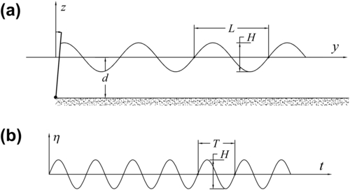
A vertical plate swinging periodically at one end of a channel generates waves on the free surface. If we take a photo of the water surface, we get a picture of the surface elevation η as a function of abscissa y along the propagation axis (the channel's axis). Function η(y) at a fixed instant represents the waves on the space domain (see Fig. 1.2(a)). If we record the surface elevation at a fixed point as a function of time t, we get the waves on the time domain (see Fig. 1.2(b)).
From Fig. 1.2(a) and (b) of the waves on the space domain and on the time domain, we get the definitions of the basic parameters: wave height H, which is the vertical distance between the highest and the lowest surface elevation in a wave; wavelength L, which is the interval between one zero up-crossing and the next of the wave on the space domain; and wave period T, which is the interval between one zero up-crossing and the next one of the wave on the time domain. Besides these three parameters, it is convenient to define the wave steepness, which is the ratio H/L, and moreover
FIGURE 1.2(a) Waves on the space domain. (b) Waves on the time domain.
1. the wave amplitude
a≡H/2
(1.12)
2. the angular frequency
ω≡2π/T
(1.13)
3. the wave number
k≡2π/L
(1.14)
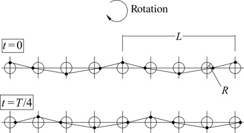
The scheme of Fig. 1.3 should be useful to understand the wave motion. Each point in the figure moves along a circular orbit, with constant speed. The time taken to cover the orbit (circumference) is T, and the figure shows two instant pictures taken at a time interval of T/4 from each other. The line connecting the points represents a wave. We see the wave advance of L/4 in a time interval of T/4, and this means that the phase speed of the wave is
c=L/T
(1.15)
The speed v of each point is generally different from c; indeed,
v=2πR/T
(1.16)
FIGURE 1.3Each point covers a circular orbit of radius R in a time T; the line connecting the points is a wave whose propagation speed is L/T.
1.3. Stokes' Theory to the First Order
Let us fix period and swinging amplitude, and let us set the wavemaker in motion. Waves with a height H1 will form.
Let us stop the wavemaker, and let us set the engine in a different manner: the same period, a smaller swinging amplitude. Then let us start again. Waves with a height H2 smaller than H1 will form. The wave period will be the same as before. Indeed, the wave period proves to be the same as the period of the wavemaker.
Let us repeat the process many times—each time with the same period T and with wave heights smaller and smaller. Doing so, in the first wave generations, which are the ones with the greater heights, we shall note asymmetry between the wave crest and trough: the crest will be steeper than the trough. Then, we shall find that a gradual lowering of the wave height, under the same period, leads to waves with a smaller asymmetry; the wave approaches a sinusoidal wave with a wavelength that depends on d and T.
Summarizing:
asH→0(dandTfixed):η(y,t)=H2cos(2πLy−2πTt)
(1.17)
where, for the moment, wavelength L is unknown. Function (1.17) represents a periodic wave of length L on the space domain and it represents a periodic wave of period T on the time domain. The negative sign in the cosine implies that the wave travels along the y-axis (with a positive sign the wave would travel in the opposite direction).
Generating waves with smaller and smaller heights (and a fixed period), we shall also note that the velocity components, at any fixed depth, will tend to fluctuate in space–time like η(y,t): vy in phase with η and vz with some phase angle. Moreover, the particle velocity will prove to be proportional to the wave height.
From these observations on particle velocity, we can draw the following identikit of the velocity potential:
where f1(z; d, T, L) denotes a function of z, wherein parameters d, T, and L may generally be present. For the moment, functions f1 and f2 and phase angle ε are unknown.
The Eqns (1.17) and (1.18) show that both η and ϕ are infinitesimal of order H. In particular, the fact that η is infinitesimal enables us to rewrite Eqns (1.6) and (1.7) in the form
where the value of a function at z=η has been expressed as: (value of the function at z=0)+(value of the derivative with respect to z, at z=0)×η. Neglecting the terms of orders smaller than or equal to H2, Eqns (1.19) and (1.20) may be reduced to
(∂ϕ∂t)z=0=−gη+1ρf(t)
(1.21)
(∂ϕ∂z)z=0=∂η∂t
(1.22)
There is only one form of ϕ (y, z, t)—Eqn (1.18)—that satisfies Eqns (1.8), (1.9) and (1.21). This is
There remains Eqn (1.22) to be satisfied, and this implies the existence of the following relationship among wavelength, water depth, and wave period:
L=gT22πtanh(2πdL)
(1.24)
This is the dispersion relationship. For calculating L by means of this relationship, it is convenient to define the sequence
Li=L0tanh(2πdLi−1)
(1.25)
with
L0≡gT22π
(1.26)
The sequence converges, and it can be easily verified that
Li<Lifiisanoddnumber
(1.27)
Li>Lifiisanevennumber
(1.28)
Hence, L is the limit of the sequence.
Since f(t) is an arbitrary function of time, the velocity potential Eqn (1.23) is indeterminate. However, the functions that are of interest, that is to say v(y, z, t) and p(y, z, t), prove to be independent of f(t), and thus they are definite. In particular, the components of vector v proceed through Eqns (1.1) and (1.2) and prove to be
vy(y,z,t)=gH2ω−1kcosh[k(d+z)]cosh(kd)cos(ky−ωt)
(1.29)
vz(y,z,t)=gH2ω−1ksinh[k(d+z)]cosh(kd)sin(ky−ωt)
(1.30)
As to the pressure, it is obtained by means of the Bernoulli Eqn (1.5). The result is
p(y,z,t)=−ρgz+ρgH2cosh[k(d+z)]cosh(kd)cos(ky−ωt)
(1.31)
(where the terms of order smaller than or equal to H2 have been neglected).
1.4. Stokes' Theory to the Second Order
Surface elevation and velocity potential can be expressed in the form
η≡η′+η″+o(H2),ϕ≡ϕ′+ϕ″+o(H2)
(1.32)
where η′ and ϕ′ are the terms of order H, the formulas of which are, respectively, Eqns (1.17) and (1.23), η″ and ϕ″ are the terms of order H2 that we shall obtain in what follows, and o(H2) is for terms of order smaller than H2, that is, terms of order H3, H4, and so on.
This is the form exact to the order H2 of one term of the system of Eqns (1.6)–(1.9). Similarly, we can also write the form exact to the order H2 of the other terms of the aforesaid system of equations. The result is
where the framed terms form the linear equations that are satisfied if η′ and ϕ′ are given by Eqns (1.17) and (1.23). Therefore, the framed terms can be canceled.
In order to solve the system Eqns (1.34)–(1.37) of the two unknown functions η″ and ϕ″, we may differentiate with respect to time all the terms of Eqn (1.34), multiply by g all the terms of Eqn (1.35), and finally add Eqn (1.35) to Eqn (1.34); in doing so we eliminate η″; that is, we obtain an equation with only the unknown function ϕ″, and the known functions η′ and ϕ′. Then, substituting η′ and ϕ′ by their expressions Eqns (1.17) and (1.23), we get
Therefore, function ϕ″ must satisfy this equation proceeding from Eqns (1.34) and (1.35), as well as the Eqns (1.36) and (1.37). The solution is a function of the kind
ϕ″(y,z,t)=Acosh[2k(d+z)]sin[2(ky−ωt)]+Bt+Cy
(1.39)
where A, B, and C are unknown constants. Substituting this expression of ϕ″ in Eqn (1.38), we get
A=332H2ω1sinh4(kd)
(1.40)
At this stage, having obtained the expression of ϕ″ (apart from constants B and C), we can obtain the expression of η″ by means of Eqn (1.34). The result is
Constant B can then be obtained given that the mean surface elevation is zero, so that the water mass in the tank is the same under the wave motion and when it is calm.
where constant C is obtained from the condition that the average flow in the waveflume is zero.
F1(kd) (function (1.42)) is positive all over its domain, and, as a consequence, the sum of η″ and η′ leads to a wave profile like that of Fig. 1.4: the crest sharpens and the trough flattens. Thus, the nonlinear theory succeeds in predicting the characteristic asymmetry between crest and trough (see Section 1.3).
FIGURE 1.4The second-order term η″ makes the wave crest steeper and flattens the wave trough.
The second-order term of the fluctuating pressure head is
Δp″γ=−1g∂ϕ″∂t−12g[(∂ϕ′∂y)2+(∂ϕ′∂z)2]
(1.45)
Here, note that the kinetic term (that is, the second addendum on the RHS of this equation) is always negative. Hence, because of the kinetic term, the fluctuating pressure head at some depth (especially on deep water) may have an asymmetry trough/crest opposite to that of the surface waves.
1.5. Wave–Current Interaction
Let us consider a periodic wave traveling on a current of speed u, in the limit H→0 for fixed d, T, and u. Let us assume the current velocity to be parallel to the wave propagation. The current direction can be the same or opposite to the direction of wave advance; that is, u may be positive or negative.
The surface elevation will have the same form Eqn (1.17) valid in absence of current, except for a different relation between wave number and water depth and wave period; that is,
η(y,t)=H2cos(kcy−ωt)
(1.46)
where kc is the wave number generally different from k, which must be determined. This new wave number will depend not only on d and T, but also on u. As to the velocity potential, it will be the sum of two terms: one of the uniform current and one like Eqn (1.23) (the velocity potential of a wave without current). Accordingly, we write
where A is a dimensional constant and F(t) a function of time, both of which need to be determined. Without the current (u=0), A is equal to gH2ω−1. Naturally, with the current, A will depend on u.
Let us seek kc, A, and F(t) such that η and ϕ satisfy the differential Eqns (1.6)–(1.9) of general validity. As to Eqns (1.8) and (1.9), it is easy to verify that they are satisfied whatever the kc, A, and F(t). Let us now pass to Eqns (1.6) and (1.7). This time ∂ϕ/∂y is the sum of a finite term u and of a term of order H due to the wave. Therefore, the terms
(∂ϕ∂y)2z=ηand(∂ϕ∂y)z=η∂η∂y
respectively, of Eqn (1.6) and of Eqn (1.7), are no longer negligible to Stokes' first order, and these equations yield
1.6. Preliminary Remarks on Three-Dimensional Waves
The surface elevation of a wave whose propagation direction makes an arbitrary angle θ with y-axis is given by
η(x,y,t)=H2cos(kxsinθ+kycosθ−ωt)
(1.56)
To prove this, let us imagine a point moving with a uniform speed L/T along a straight line making an angle θ with the y-axis. If the point starts from x=0, y=0 at time t=0, its position is given by
xP=LTtsinθ,yP=LTtcosθ
(1.57)
so that the surface elevation at this point proves to be
η(xP,yP,t)=H2cos(2πTtsin2θ+2πTtcos2θ−2πTt)=H2
(1.58)
and hence, it keeps constant in time, which confirms that the trajectory and speed of the wave is coincident with the trajectory and speed of the point.
The velocity potential attacked to surface elevation Eqn (1.56) is
Here, we can readily verify that the two functions (1.56) and (1.59) satisfy Eqns (1.21) and (1.22), provided that f(t)=0 in Eqn (1.21), as well as the boundary condition at the bottom; see Eqn (1.9). Note: These equations, having been obtained for the two-dimensional flow y-z, retain their validity even for the three-dimensional flow x-y-z. As to f(t)=0, we have already seen that v and p do not change whatever the f(t), and therefore it is justified and advisable to put directly f(t)=0 in Eqn (1.21).
Of the whole system of linear flow equations, that is, the system consisting of Eqns (1.8) and (1.9) and Eqns (1.21) and (1.22), the only equation that needs to be adjusted from the two-dimensional to the three-dimensional flow is Eqn (1.8). For the three-dimensional flow, it becomes
Let us consider the flow field if a wave train attacks a long vertical breakwater. Let us assume that the breakwater is along line y=0, and the direction of the incident waves makes an angle θ with the y-axis (see Fig. 1.5).
On the ground of some intuitive considerations, we could at once say that specular reflection will occur and that the height and period of the reflected waves will be equal to the height and period of the incident waves; but we believe it to be useful to prove such intuitive knowledge. Therefore, we assume that the direction of the reflected waves makes an unknown angle ˜θ with the y-axis, and in addition, we allow the possibility that the reflected waves may have a height ∼H and a period ˜T different from height H and period T of the incident waves.
The η and ɸ of the incident waves are given by Eqns (1.56) and (1.59), and the η and ɸ of the reflected waves are given by the same equations with ˜H, ˜ω, ˜k, and ˜θ in place of H, ω, k, and θ:
We cannot exclude some phase angle between the reflected and the incident waves, and this is why in the expressions of the reflected waves we have put a phase angle ε that must be determined.
FIGURE 1.5Reflection: reference scheme.
The flow field before the wall is given by the sum of the incident waves (Eqns (1.56) and (1.59) of η and ɸ) and of the reflected waves (Eqns (1.61) and (1.62)):
In the basic case of θ=0, in which the wave attacks the breakwater orthogonally, the flow becomes two-dimensional y-z and the formulas of η and ɸ reduce themselves to
Three instant pictures of this basic case are given in Fig. 1.6.
At time t=0, both vy and vz are zero everywhere, given that both vy and vz are proportional to sin(ωt). At that time (t=0), the surface elevation gets to its maximum (positive or negative) at each location. In particular, at the wall, the surface elevation at t=0 is equal to the crest-to-trough height of the incident wave.
FIGURE 1.6Three snapshots of the wave field before a vertical breakwater.
At time t=T/4, the surface elevation is zero everywhere, given that η is proportional to cos(ωt). The horizontal velocity has its negative maximum at y=−L/4, and it has its positive maximum at y=−34L. The vertical velocity has its negative maximum at the wall (y=0) and at y=−L, and it has its positive maximum at y=−L/2.
At time t=T/2, the surface elevation is opposite with respect to the surface elevation at t=0. Thus, a consistent picture emerges, where:
1. at time t=0, the water surface is higher than the MWL in sections ① and ④, and is lower than the mean water level (MWL) in sections ② and ③ (Fig. 1.6);
2. vice-versa, at time t=T/2 the water surface is lower than the MWL in sections ① and ④, and is higher than the MWL in sections ② and ③;
3. consistently, at the intermediate time instant t=T/4, the water flows from sections ① and ④ toward sections ② and ③.
There are some points (nodes) where the surface elevation is always zero, and where the horizontal velocity attains its absolute maximum. These points are at 14, 34, 54, … wavelengths from the wall. Then there are the antinodes, at 0, 12, 1, 32, … wavelengths from the wall, where the wave height (on the time domain) and the vertical velocity attain their absolute maximum.
The wave height in the time domain at the antinodes is 2H, which is twice the wave height that would be there without the wall. The velocity maxima are also twice the maxima in the absence of the wall.
1.7.3. The Pressure Distribution on the Breakwater
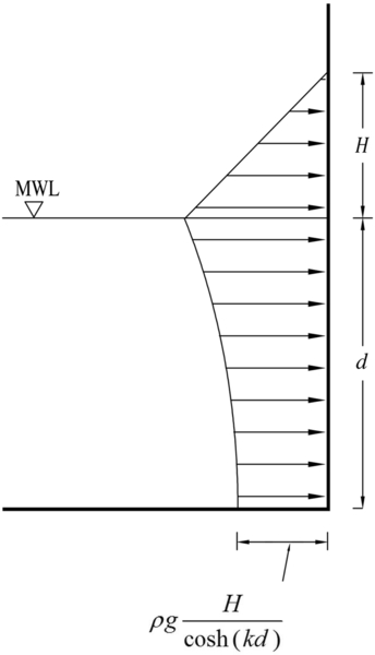
Whichever the angle θ of the waves, the maximum pressure at any fixed section of the breakwater, according to Stokes' first order, is given by
p(z)=−ρgz+ρgHcosh[k(d+z)]cosh(kd)
(1.74)
which proceeds from Eqn (1.69) of ɸ, and can be rewritten in the equivalent form (apart from a term of order H2):
FIGURE 1.7The pressure exerted on a vertical breakwater by a wave crest.
The wave pressure, that is, the difference between the actual pressure and the static pressure, is shown in Fig. 1.7.
For the formal step from Eqns (1.74)–(1.76), note that
Hcosh[k(d+z)]cosh(kd)=H+o(H)if0<z<H
(1.77)
1.8. Wave Diffraction
1.8.1. Interaction with a Semi-infinite Breakwater
Let us consider a vertical breakwater along the line y=0, with the origin at x=0 and negligible thickness. The flow field that would be there without the breakwater is the one given by formulas (1.56) and (1.59) of η and ɸ.
From the solution of Penney and Price (1952), the surface elevation and the velocity potential to Stokes' first order, in polar coordinates, are given by
Let us arbitrarily fix a point r, β and let us write F and G in place of F(r, β, ω, θ) and G(r, β; ω, θ). The surface elevation on the time domain, at the fixed point, has its maxima and minima at times tm such that
ωtm=arctan(GF)
(1.86)
FIGURE 1.8Reference scheme for the interaction between waves and a semi-infinite breakwater.
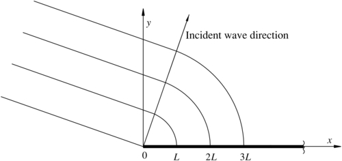
FIGURE 1.9Wavefronts behind a semi-infinite breakwater.
Therefore, tm1 is the time instant of the crest and tm2 is the time instant of the trough at the fixed point. Clearly, instants tm1 and tm2 generally change from one point to another since they depend on functions F and G. The wavefronts (see Fig. 1.9) are the lines connecting points with the same value of tm1 (or tm2).
1.8.2. The Diffraction Coefficient
From Eqn (1.89), it follows that the wave height (that is, the height of the wave on the time domain) is
H(r,β)=H√F2+G2
(1.90)
As a consequence, the diffraction coefficient, which is defined as the quotient between the wave height at a given point and the height of the incident waves, is given by
Cd(r,β)=√F2+G2
(1.91)
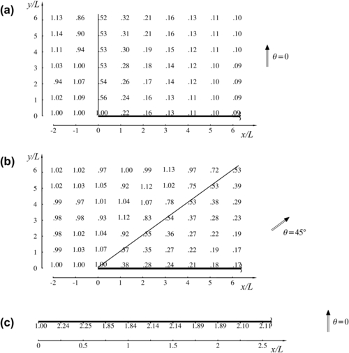
FIGURE 1.10Diffraction coefficient.
(a) Behind the breakwater (orthogonal wave attack), (b) behind the breakwater (inclined attack), and (c) along the wave-beaten wall (orthogonal attack).
The Cd for two different angles of the wave direction are given in Fig. 1.10(a) and (b). Of course, the diffraction coefficient at the sheltered side of the breakwater gets smaller and smaller with the distance from the tip of the breakwater. At the wave-beaten side of the breakwater (β=2π), Cd takes on a maximum somewhat greater than 2.0, close to the tip of the breakwater (Fig. 1.10(c)).
1.9. Energy Flux and Wave Energy
Let us consider a y-z flow, with y being the wave direction. The mean energy flux per unit length is given by
Φ=〈η∫−d[p+ρgz+12ρ(v2y+v2z)]vydz〉
(1.92)
where the angle brackets denote an average with respect to time t. With Eqn (1.31) of p and Eqn (1.29) of vy, and neglecting the terms of an order smaller than H2, we get
Finally, multiplying and dividing the RHS by sinh(kd), it follows that
Φ=ρgH28c2[1+2kdsinh(2kd)]
(1.97)
where use has been made of the equation of the phase speed
c=LT=gT2πtanh(kd)
(1.98)
Let us pass to the equation of the mean wave energy per unit surface. This is
E=〈η∫0ρgz〉+〈η∫−d12ρ(v2y+v2z)dz〉
(1.99)
where, neglecting the terms of order smaller than H2, and performing a few steps like those we have done for obtaining the compact form of Ф, we arrive at
E=18ρgH2
(1.100)
1.10. The Group Velocity
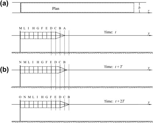
Let us assume that the wavemaker of a waveflume is switched. Initially, we would see some waves close to the wavemaker with the rest of the waveflume still being calm. Then, we would see the wave zone widen gradually. We have
1. average energy entering the CV of Fig. 1.11(a) in the unit time=Фb,
2. average increment of the wave energy in the CV in the unit time=EbcG,
FIGURE 1.11(a) Plan view of a waveflume and control volume for the deduction of Eqn (1.102) of cG. (b) Three pictures taken a wave period from each other, while the wave motion advances on an initially still basin (the waves are sketched as vertical segments).
where cG is the propagation speed of the wave motion on the waveflume. Hence,
Here, it can be readily verified that cG is generally smaller than c, and on deep water, cG is half the c. Let us see the reason for this.
Figure 1.11(b) shows three instant pictures of the waveflume taken an interval T from each other. The waves are sketched as vertical segments; the height of the segment is equal to the wave height and the interval between two consecutive segments is equal to the wavelength. Each single wave advances a wavelength L in a wave period T, so that its propagation speed (phase speed) is L/T. It is not so for the wave group that advances by a wavelength in two wave periods, so that its propagation speed is c/2. The propagation speed of the group is smaller than the propagation speed of each single wave, simply because each single wave goes to die at the group head. In particular, in the first picture, wave A is going to die; then in the third picture, two periods later, wave B is going to die; then it will be the turn of C, D, and so on. (Of course, the envelope front in Fig. 1.11(b) has been somewhat simplified.)

 (1.6)
(1.6) (1.10)
 (1.11)
 (1.19)
 (1.23)

 (1.51)
 (1.52)
 (6.61)
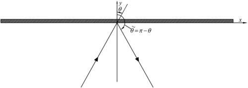
 (1.64)
 (1.66)
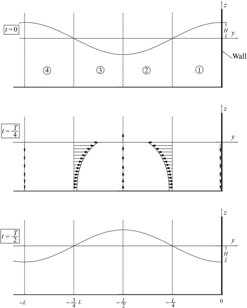
 (1.83)
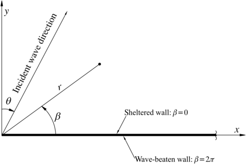
 (1.92)
 (1.93)
 (1.94)
 (1.95)
 (1.99)