Search in book...
Toggle Font Controls
Create new playlist

Name your new playlist

Playlist description (optional)
Sign In

Email address

Password

Forgot Password?

or

Continue with Facebook

Continue with Google
Sign Up

Full Name

Email address

Confirm Email Address

Password

or

Continue with Facebook

Continue with Google

Chapter 14

Loads of Sea Storms on Vertical Breakwaters

Abstract

The chapter starts from the equilibrium problem of a caisson breakwater, and it recalls how stability is examined. It shows Goda's model (GM) for the estimate of the largest load in a given sea state. Then, the chapter introduces fresh results of an extensive small-scale field experiment. These results support GM for the positive wave loads. As for the negative wave loads (those exerted by wave troughs), the chapter suggests using the linear theory with a virtual wave height. The chapter concludes with two worked examples of vertical breakwaters on water depth of, respectively, of 18 and 54 m.

Keywords

Goda's model; Small-scale field experiment (SSFE); Vertical breakwater; Wave load

14.1. Overall Stability of an Upright Section

14.1.1. The Equilibrium Problem

The wave pressures on an upright section (caisson + concrete crown), under a wave crest and a wave trough, are shown in Fig. 14.1.

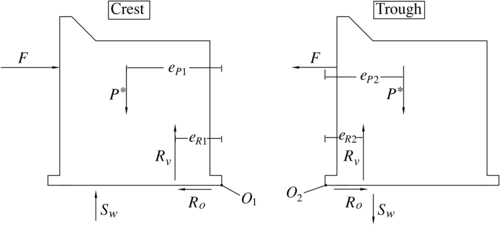
Figure 14.2 shows the forces on the upright section: weight P^∗ in still water, wave forces F and S_w, and horizontal and vertical reactions R_o and R_v of the rubble mound. For the equilibrium, we have

$| R_{o} | = | F |$ $| R_{o} | = | F |$

(14.1)

$R_{v} = P^{*} - S_{w}$ $R_{v} = P^{*} - S_{w}$

(14.2)

where the uplift force S_w is positive under the wave crest and negative under the wave trough. The position of R_v is such that the free body is in equilibrium:

$M + R_{v} e_{R} = P^{*} e_{P}$ $M + R_{v} e_{R} = P^{*} e_{P}$

(14.3)

with M being the overturning moment due to wave forces F and S_w (under a wave trough, S_w gives a negative contribution to M). Under a wave crest, the topple axis is O₁ so that e_P = e_P1 and e_R = e_R1; and under a wave trough, the topple axis is O₂ so that e_P = e_P2 and e_R = e_R2.

FIGURE 14.1 Wave pressure on the wall and on the base of an upright breakwater.

FIGURE 14.2 Reference scheme for the stability analysis.

A static analysis of the upright section with the extreme wave load is usually done, at least for preliminary design purposes. The stability of the upright section is examined for three modes of failure.

Against sliding. We must verify that the safety factor

$C_{1} \equiv \frac{μ R_{v}}{| R_{o} |} = \frac{μ (P^{*} - S_{w})}{| F |}$ $C_{1} \equiv \frac{μ R_{v}}{| R_{o} |} = \frac{μ (P^{*} - S_{w})}{| F |}$

(14.4)

is greater than some dictated value C_1 min >1. μR_v (friction coefficient × vertical reaction) is the limit shear force that can be developed at the base of the caisson. Thus, we check that the limit horizontal reaction (that the rubble mound can exert) is suitably greater than the actual horizontal reaction the rubble mound is expected to exert.

Against overturning. We must verify that the safety factor

$C_{2} \equiv \frac{P^{*} e_{P}}{M}$ $C_{2} \equiv \frac{P^{*} e_{P}}{M}$

(14.5)

is greater than some dictated value C_2 min >1. Indeed, were P^∗e_P equal to M, then e_R would be zero (cf. Eqn (14.3)), and hence the overturning would occur. Then, C_2 min should be greater than C_1 min, given that C₁ can approach 1 without breakwater sliding, while a failure will occur certainly before than C₂ approaches 1. This will be the collapse of foundation, given that as C₂ approaches 1, e_R approaches zero, and hence the bearing pressure at O₁ tends to infinity.

Against collapse of foundation. A common procedure is to check that the largest toe pressure is within 4·10⁵ ÷ 5·10⁵ N/m². An alternative way may be verifying that the safety factor

$C_{3} \equiv \frac{B_{C}}{R_{v} / 2 e_{R}}$ $C_{3} \equiv \frac{B_{C}}{R_{v} / 2 e_{R}}$

(14.6)

is greater than some dictated value C_3 min >1. The denominator on the RHS of this formula gives the bearing pressure, and the numerator (B_C) represents the bearing capacity, which depends on the characteristics of the soil, on the ratio R_o/R_v, and on e_R.

The verifications of the stability against overturning and against collapse of foundation really aim to check the stability against one mode of failure: under the wave force, e_R is reduced so that the bearing pressure at the heel of upright section becomes too large, the soil collapses and the structure tilts and sinks into the ground.

14.2. Wave Pressures

14.2.1. Goda's Model

Following Goda (2000), the H_s and H for the design of a breakwater are

$H_{s} = C_{s} H_{s_{0}} if d_{n} / L_{0} > 0.2$ $H_{s} = C_{s} H_{s_{0}} if d_{n} / L_{0} > 0.2$

(14.7)

$H_{s} = Min (β_{0} H_{s_{o}} + β_{1} d_{n}, β_{\max} H_{s_{o}}, C_{s} H_{s_{o}}) if d_{n} / L_{0} < 0.2$ $H_{s} = Min (β_{0} H_{s_{o}} + β_{1} d_{n}, β_{\max} H_{s_{o}}, C_{s} H_{s_{o}}) if d_{n} / L_{0} < 0.2$

(14.8)

$H = 1.8 C_{s} H_{s_{0}} if d_{n} / L_{0} > 0.2$ $H = 1.8 C_{s} H_{s_{0}} if d_{n} / L_{0} > 0.2$

(14.9)

$H = Min ({\hat{β}}_{0} H_{s_{0}} + {\hat{β}}_{1} d_{n}, {\hat{β}}_{\max} H_{s_{0}}, 1.8 C_{s} H_{s_{0}}) if d_{n} / L_{0} < 0.2$ $H = Min ({\hat{β}}_{0} H_{s_{0}} + {\hat{β}}_{1} d_{n}, {\hat{β}}_{\max} H_{s_{0}}, 1.8 C_{s} H_{s_{0}}) if d_{n} / L_{0} < 0.2$

(14.10)

where C_s is the shoaling coefficient: the terms β are due to dissipation of wave energy, with β₀, β₁, β_max, and

{\hat{β}}_{0}, {\hat{β}}_{1}, {\hat{β}}_{\max},

${\hat{β}}_{0}, {\hat{β}}_{1}, {\hat{β}}_{\max},$

depending on sea bottom slope λ, and β₀, β_max,

{\hat{β}}_{0}, {\hat{β}}_{\max},

${\hat{β}}_{0}, {\hat{β}}_{\max},$

also depending on the wave steepness H_s0/L₀. If there is refraction and/or diffraction from deep water to water depth d_n,

H_{s_{0}}

$H_{s_{0}}$

must be intended as the actual deep water significant wave height multiplied by the diffraction coefficient (C_d) and the refraction coefficient (C_r). C_d is estimated by means of Eqn (7.50), and C_r by means of a similar equation based on the deep water directional spectrum.

The distribution of wave pressure on the wall and on the base is given by the following equations, wherein reference is made to Fig. 14.3:

$η_{\max} = \frac{3}{4} (1 + \cos θ) H$ $η_{\max} = \frac{3}{4} (1 + \cos θ) H$

(14.11)

$p_{w_{1}} = \frac{1}{2} (1 + \cos θ) (α^{'} + α^{″} \cos^{2} θ) γ H$ $p_{w_{1}} = \frac{1}{2} (1 + \cos θ) (α^{'} + α^{″} \cos^{2} θ) γ H$

(14.12)

$p_{w} = α^{‴} p_{w_{1}}$ $p_{w} = α^{‴} p_{w_{1}}$

(14.13)

$p_{w_{2}} = \frac{1}{2} (1 + \cos θ) α^{'} α^{‴} γ H$ $p_{w_{2}} = \frac{1}{2} (1 + \cos θ) α^{'} α^{‴} γ H$

(14.14)

where

$α^{'} = 0.6 + \frac{1}{2} {[\frac{2 k d_{n}}{\sinh (2 k d_{n})}]}^{2}$ $α^{'} = 0.6 + \frac{1}{2} {[\frac{2 k d_{n}}{\sinh (2 k d_{n})}]}^{2}$

(14.15)

$α^{″} = Min [(\frac{d_{n}^{'} - d}{3 d_{n}^{'}}) {(\frac{H}{d})}^{2}, 2 \frac{d}{H}]$ $α^{″} = Min [(\frac{d_{n}^{'} - d}{3 d_{n}^{'}}) {(\frac{H}{d})}^{2}, 2 \frac{d}{H}]$

(14.16)

$α^{‴} = 1 - \frac{d^{'}}{d_{n}} [1 - \frac{1}{\cosh (k d_{n})}]$ $α^{‴} = 1 - \frac{d^{'}}{d_{n}} [1 - \frac{1}{\cosh (k d_{n})}]$

(14.17)

where

d_{n}^{'}

$d_{n}^{'}$

denotes the water depth at a distance of 5H_s seawards of the breakwater. Cautiously, it is suggested that the wave direction is rotated by an amount of up to 15° toward the line normal to the breakwater from the principal wave direction.

FIGURE 14.3 Reference scheme for Goda's model (GM).

As to the wave period, Goda uses T_1/3, that is, the average period of the largest 1/3 waves of the sea state. This period proves to be very close to T_h—the wave period of very large waves, which proceeds from the autocovariance (see Section 4.5.1). In an SSFE on 750 sea states consisting of wind seas, the average T_1/3/T_h was equal to 0.994 (cf. Boccotti et al., 2012). As for the negative wave pressures, under wave troughs, Goda (2000) supplies a diagram (see his Fig. 4.9) that enables one to estimate the resultant force for given wave height and period and water depth.

14.2.2. The Virtual-Height Model

Nonlinearity effects yield some characteristic deformation of wave pressure at a breakwater (without changing the overall configuration of wave groups). Roughly, it is as if the positive pressures were those of a linear wave, and the negative pressures were those of a linear wave with a larger height. This is what emerged from the SSFE described in Chapter 13 of a previous book. As a consequence, the following model was suggested for the largest positive pressures and the largest negative pressures, respectively, of a given sea state

$wave crest Δ p = {\begin{matrix} γ H^{+} \frac{\cosh [k (d + z)]}{\cosh (k d)} & if z \leq 0 \\ γ^{(H^{+} - z)} & if z > 0 \end{matrix}$ $wave crest Δ p = {\begin{matrix} γ H^{+} \frac{\cosh [k (d + z)]}{\cosh (k d)} & if z \leq 0 \\ γ^{(H^{+} - z)} & if z > 0 \end{matrix}$

(14.18)

$wave trough Δ p = {\begin{matrix} - γ H^{-} \frac{\cosh [k (d + z)]}{\cosh (k d)} & if Δ p > - p_{i d} \\ - p_{i d} & otherwise \end{matrix}$ $wave trough Δ p = {\begin{matrix} - γ H^{-} \frac{\cosh [k (d + z)]}{\cosh (k d)} & if Δ p > - p_{i d} \\ - p_{i d} & otherwise \end{matrix}$

(14.19)

Equation (14.18) gives the average pressure distribution of a given share of the largest positive peaks of the horizontal force on the breakwater. Equation (14.19) gives the average pressure distribution of a given share of the largest negative peaks of the horizontal force on the breakwater. In these equations, H⁺ and H⁻ are virtual wave heights that depend on whether the given share is, for example, 1/1000 or 1/100. In particular,

$H^{+} = 1.40 H_{s}, H^{-} = 2.31 H_{s}$ $H^{+} = 1.40 H_{s}, H^{-} = 2.31 H_{s}$

(14.20)

with the 1/1000 largest waves of a sea state.

14.3. Evidences from SSFEs

The SSFE of Boccotti (2000) covered only the range 0.15 < d/L_p0 < 0.20. An SSFE covering a wider range of d/L_p0 was performed in 2009—see Fig. 14.4. For the aims of the following synthesis:

F⁺ will be the average of the 1/1000 share of the largest positive force peaks measured in a sea state;

F_{G M}^{+}

$F_{G M}^{+}$

, the largest positive wave force in a sea state, calculated according to the GM;

FIGURE 14.4 The vertical breakwater used for the SSFE of 2009 on a wide range of d/L_p0.
Water depth d was equal to 1.88 m + tide level. The tide amplitude was within 0.16 m.

F_{V H M}^{+}

$F_{V H M}^{+}$

, the average of the 1/1000 share of the largest positive force peaks in a sea state calculated according to the virtual-height model (VHM);

F⁻,

F_{G M}^{-}, and F_{V H M}^{-},

$F_{G M}^{-}, and F_{V H M}^{-},$

will have the same meaning as F⁺,

F_{G M}^{+}, and F_{V H M}^{+},

$F_{G M}^{+}, and F_{V H M}^{+},$

with the only difference to represent the absolute values of the force exerted by a wave trough instead of the force exerted by a wave crest.

F_{G M}^{-}

$F_{G M}^{-}$

is based on the abacus of Fig. 4.9 of the book of Goda (2000), with H given by Eqn (14.10).

F_{G M}^{+}, F_{V H M}^{+}, F_{G M}^{-}, and F_{V H M}^{-}

$F_{G M}^{+}, F_{V H M}^{+}, F_{G M}^{-}, and F_{V H M}^{-}$

were obtained from the H_s, T_h or T_1/3 of the measured incident waves.

The following emerges from the SSFE of 2009:

F_{G M}^{+}

$F_{G M}^{+}$

is a 3% smaller than F⁺ on the range (0.10 < d/L_p0 < 0.15),

F_{G M}^{+}

$F_{G M}^{+}$

is greater than F⁺, of 7–9%, on the range (0.15 < d/L_p0 < 0.25),

F_{V H M}^{+}

$F_{V H M}^{+}$

with the virtual wave height H⁺ of 1.4 H_s underestimates F⁺ from the 5% to the 10%,

F⁻ is smaller than F⁺ for d/L_p0 < 0.15,

F⁻ is equivalent to F⁺ for 0.15 < d/L_p0 < 0.20,

F⁻ is greater than F⁺ for d/L_p0 > 0.20

which implies that the verification of the stability under wave trough usually becomes important only for d/L_p0 > 0.20. Hence, we focus negative wave forces only on this range, where the picture is the following:

F_{G M}^{-}

$F_{G M}^{-}$

is about the 20% smaller than F⁻, on 0.20 < d/L_p0 < 0.30,

whereas

F_{V H M}^{-}

$F_{V H M}^{-}$

with

$H^{-} = 3.0 H_{s} on the range 0.20 < d / L_{p 0} < 0.30$ $H^{-} = 3.0 H_{s} on the range 0.20 < d / L_{p 0} < 0.30$

(14.21)

gives a nearly perfect agreement with the measured pressure distributions.

The wide (though not exhaustive) test of the 2009 SSFE suggests that the GM is being widely used and yielding forces that are close to, or somewhat greater than, F_1/1000, and continue to be used for estimating positive pressure on vertical breakwaters. On the other hand, the VHM, with some appropriate values of the virtual wave height H⁻, is effective for estimating negative pressures.

14.4. The Risk of Impulsive Breaking Wave Pressures

If the breaking point of a progressive wave (in the absence of a structure) is located only slightly in front of the breakwater, or the combined sloping section and top berm of the rubble mound is rather broad, there may be danger of impulsive breaking wave pressure. Following Goda (2000), if the rubble mound is sufficiently small enough to be considered negligible, then there is little danger of impulsive breaking wave pressure if at least one of the following conditions occur:

1. the sea bottom slope being smaller than 0.02,

H_{s_{0}} C_{r} C_{d} / L_{0}

$H_{s_{0}} C_{r} C_{d} / L_{0}$

being greater than 0.03 (L₀ being the deep water wave length corresponding to T_h),

3. the crest elevation of the wall allowing much overtopping.

A recent (May 2013) SSFE performed in the NOEL under my direction (results still unpublished) has evidenced that impulsive breaking wave pressures may occur even if both conditions (2) and (3) are fulfilled. However, the experiment has also shown that caisson breakwaters may resist unexpectedly well to these impulsive forces, whereas breakwaters consisting of solid concrete blocks collapse in line with the expectation. The high resistance of caissons should be due to the effect of mound foundation and ground, which are elastically deformed under the application of an impulsive wave breaking pressure (see Goda, 1992). This research is in due course: the configuration of the lee side of the rubble mound could prove to be important.

14.5. Worked Examples

14.5.1. First Worked Example

Vertical breakwater with d = 14 m, W = 7 m, d^' = 15.5 m, d_n = 18 m, λ = 0.02, straight contour lines; design sea state:

H_{s_{0}} = 8.0 m,

$H_{s_{0}} = 8.0 m,$

spectrum: mean JONSWAP with A = 0.01; directional distribution: Mitsuyasu et al. with n_p = 20 and θ_d = 0.

Results of calculations (GM applied): T_p = 12.1 s, T_h = 11.1 s, H_s = 7.18 m, H = 12.9 m, η_max = 19.3 m,

p_{w_{1}} = 114 {kN/m}^{2}

$p_{w_{1}} = 114 {kN/m}^{2}$

, p_w = 87 kN/m², F⁺ = 2210 kN/m.

This is a case in which impulsive pressure could occur, and their intensity should be sensitive to the berm width (for a deeper insight into this item, see the questionnaire, Table 4.1 of Goda, 2000; prepared by referring to Tanimoto's examination).

The ratio d/L_p0 (=0.06) is smaller than 0.20, hence the negative wave force is expected to be smaller than the positive wave force.

14.5.2. Second Worked Example

Vertical breakwater with d = 50 m, W = 7 m, d^' = 51 m, d_n = 54 m, λ = 0.02, straight contour lines; design sea state: same deep water characteristics as for the first worked example.

Results of calculations (GM applied): T_p = 12.1 s, T_h = 11.1 s, H_s = 7.36 m, H = 13.2 m, η_max = 19.8 m,

p_{w_{1}} = 82 {kN/m}^{2}

$p_{w_{1}} = 82 {kN/m}^{2}$

, p_w = 28.4 kN/m², F⁺ = 3300 kN/m.

In this case, because of the large water depth (d/L_p0 = 0.22), it is also necessary to evaluate the effect of the wave trough. Result of calculations (VHM applied): H⁻ = 22.1 m, Δp is represented in Fig. 14.5, F⁻ = 4570 kN/m, which is definitely greater than F⁺ (=3300 kN/m).

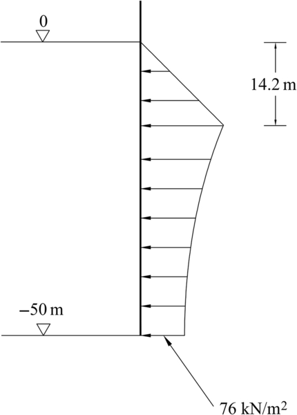
FIGURE 14.5 Second worked example, Chapter 14: negative wave pressure on a 50-m-deep breakwater.
The resultant force on (−d = −50 m < z < 0) is about 4500 kN/m. Then there is an additional small force on (−d′ = −51 m < z < −d), which is estimated to be 76 kN/m.

Notwithstanding the uplift force plays against stability under a wave crest, and pros stability under a wave trough, probably, the overall stability of this breakwater on 50-m water depth will prove to be more critical under the wave trough than under the wave crest.

14.6. Conclusion

Wave loads on vertical breakwaters are estimated with empirical formulae based essentially on waveflume data, and in part on examination of full-scale failures or nonfailures (Goda, 1974; Oumeraci, 1994). This approach is effective, and especially the great experience accumulated by the Japanese School must be exploited. A fresh contribution may come from SSFEs. The results of the SSFEs of 1994 and 2009 were disclosed, respectively, in Chapter 13 of my book (2000) and in the paper by Boccotti et al. (2012).

..................Content has been hidden....................

You can't read the all page of ebook, please click here login for view all page.

Table of Contents for Chapter 14. Loads of Sea Storms on Vertical Breakwaters

Create new playlist

Sign In

Sign Up

Abstract

Keywords

14.1. Overall Stability of an Upright Section

14.1.1. The Equilibrium Problem

14.2. Wave Pressures

14.2.1. Goda's Model

14.2.2. The Virtual-Height Model

14.3. Evidences from SSFEs

14.4. The Risk of Impulsive Breaking Wave Pressures

14.5. Worked Examples

14.5.1. First Worked Example

14.5.2. Second Worked Example

14.6. Conclusion

Table of Contents for
Chapter 14. Loads of Sea Storms on Vertical Breakwaters