Search in book...
Toggle Font Controls
Create new playlist

Name your new playlist

Playlist description (optional)
Sign In

Email address

Password

Forgot Password?

or

Continue with Facebook

Continue with Google
Sign Up

Full Name

Email address

Confirm Email Address

Password

or

Continue with Facebook

Continue with Google

Chapter 4

Wave Statistics in Sea States

Abstract

The first two sections are devoted to the basic concepts on stationary Gaussian processes. These concepts are then used to deduce Rice's solution (1958) for the expected number per unit time of b up-crossings of the random surface elevation (with b being any fixed threshold). The chapter goes on to show three corollaries of this solution, including the distribution of wave height under narrowband assumption. Then, the chapter shows some important consequences of the quasi-determinism theory on wave statistics. The conclusive part of the chapter deals with the calculation of the maximum expected wave in a sea state of given significant wave height, duration, and shape of the spectrum. Three FORTRAN programs useful for this calculation are supplied and discussed. A fresh point of view (2013) of an old subject (wave height distribution: bandwidth and third-order nonlinearity effects) is dealt with in the conclusion to the chapter.

Keywords

Average wave period; Bandwidth effect; Maximum expected wave height; Nonlinearity effect; Period largest waves; QD theory; Sea state; Small-scale field experiment (SSFE); Wave height distribution

4.1. Surface Elevation as a Stationary Gaussian Process

4.1.1. The Probability of the Surface Elevation

The random process (Eqn (3.1)) with the assumptions we have made on N, a_i, ω_i, and ε_i is stationary and Gaussian. This means that the probability p(η(t) = w)dw that η(t) of a given realization of the random process falls in a fixed small interval (w,w + dw) is equal to the probability p(η(t_o) = w)dw that η(t_o) at any fixed time instant t_o, in a realization taken at random, falls in the given interval (w,w + dw), and these have the following form:

p(η(t)=w)=p(η(to)=w)=12πm0√exp(−w22m0) $p (η (t) = w) = p (η (t_{o}) = w) = \frac{1}{\sqrt{2 π m_{0}}} \exp (- \frac{w^{2}}{2 m_{0}})$

(4.1)

The probability p(η(t) = w)dw is equal to the ratio between the time in which w < η(t) < w + dw and the total time. The probability p(η(t_o) = w)dw is equal to the ratio between the number of realizations in which w < η(t_o) < w + dw and the total number of realizations.

Now let us see how Eqn (4.1) may be achieved. First, let us consider two arbitrary random variables V₁ and V₂. If

Vn1¯¯¯¯¯=Vn2¯¯¯¯¯∀n $\bar{V_{1}^{n}} = \bar{V_{2}^{n}} \forall n$

(4.2)

reads “if the mean value of the nth power of V₁ is equal to the mean value of the nth power of V₂, whichever the n,” then the two variables have the same probability density function, that is,

p(V1=w)=p(V2=w) $p (V_{1} = w) = p (V_{2} = w)$

(4.3)

This rather intuitive property, which proceeds formally from the theorem of moments, will enable us to prove Eqn (4.1).

Before giving the proof, it is worthwhile to specify that we shall adopt two different symbols for the mean: one for the time average, the other one for the ensemble average. Specifically,

⟨ηn(t)⟩ $〈 η^{n} (t) 〉$

will denote the average of the nth power of η(t) in a given realization of the process, and

ηn(to)¯¯¯¯¯¯¯¯¯ $\bar{η^{n} (t_{o})}$

will denote the average of the nth power of η at the fixed time t_o.

4.1.2. Proof Relevant to Any Given Realization

From Eqn (3.1) and the assumption that ω_i ≠ ω_j, if i ≠ j, it follows that

⟨η4(t)⟩=3∑Ni=1∑Nj=1(j≠i)14a2ia2j+∑Ni=138a4i $〈 η^{4} (t) 〉 = 3 \sum_{i = 1}^{N} \sum_{j = 1 (j \neq i)}^{N} \frac{1}{4} a_{i}^{2} a_{j}^{2} + \sum_{i = 1}^{N} \frac{3}{8} a_{i}^{4}$

(4.4)

Here, the assumptions of Section 4.2 on N and a_i come into play (N being infinitely large, a_i being of the same order of one another). Indeed, under these assumptions, Eqn (4.4) may be rewritten in the form,

⟨η4(t)⟩=3∑Ni=1∑Nj=114a2ia2j $〈 η^{4} (t) 〉 = 3 \sum_{i = 1}^{N} \sum_{j = 1}^{N} \frac{1}{4} a_{i}^{2} a_{j}^{2}$

(4.5)

which implies

⟨η4(t)⟩=3⌊⟨η2(t)⟩⌋2=3m20 $〈 η^{4} (t) 〉 = 3 {⌊ 〈 η^{2} (t) 〉 ⌋}^{2} = 3 m_{0}^{2}$

(4.6)

Now, assuming that Eqn (4.1) is actually the probability of the surface elevation, we get the same value of

⟨η4(t)⟩ $〈 η^{4} (t) 〉$

⟨η4(t)⟩=∫+∞−∞w4p(η(t)=w)dw=12πm0√∫+∞−∞w4exp(−w22m0)dw=3m20 $〈 η^{4} (t) 〉 = \int_{- \infty}^{+ \infty} w^{4} p (η (t) = w) d w = \frac{1}{\sqrt{2 π m_{0}}} \int_{- \infty}^{+ \infty} w^{4} \exp (- \frac{w^{2}}{2 m_{0}}) d w = 3 m_{0}^{2}$

(4.7)

By the same way of reasoning, we can prove that whichever the n,

⟨ηn(t)⟩ $〈 η^{n} (t) 〉$

takes on the same value if evaluated from Eqn (3.1) of η(t) or from Eqn (4.1) of the probability of η(t). The fact that

⟨ηn(t)⟩obtainedfromEqn(3.1)=⟨ηn(t)⟩obtainedfromEqn(4.1)∀n $〈 η^{n} (t) 〉 obtained from Eqn (3.1) = 〈 η^{n} (t) 〉 obtained from Eqn (4.1) \forall n$

(4.8)

implies that Eqn (4.1) is actually the probability of η(t).

4.1.3. Proof Relevant to the Ensemble at a Fixed Time Instant

Fixing any time instant t_o, from Eqn (3.1), we have

η4(to)¯¯¯¯¯¯¯¯¯=[∑Ni=1aicos(εˆi)]4¯¯¯¯¯¯¯¯¯¯¯¯¯¯¯¯¯¯¯¯¯¯¯¯¯¯ $\bar{η^{4} (t_{o})} = \bar{{[\sum_{i = 1}^{N} a_{i} \cos ({\hat{ε}}_{i})]}^{4}}$

(4.9)

where

εˆi≡εi+ωito ${\hat{ε}}_{i} \equiv ε_{i} + ω_{i} t_{o}$

(4.10)

If the ε_i are distributed uniformly over the circle and are stochastically independent from one another, also the

εˆi ${\hat{ε}}_{i}$

are distributed uniformly over the circle and are stochastically independent from one another. Because of this property, it can be shown that

η4(to)¯¯¯¯¯¯¯¯¯=3∑Ni=1∑Nj=1(j≠i)14a2ia2j+∑Ni=138a4i $\bar{η^{4} (t_{o})} = 3 \sum_{i = 1}^{N} \sum_{j = 1 (j \neq i)}^{N} \frac{1}{4} a_{i}^{2} a_{j}^{2} + \sum_{i = 1}^{N} \frac{3}{8} a_{i}^{4}$

(4.11)

Comparing this with Eqn (4.4) of

⟨η4(t)⟩ $〈 η^{4} (t) 〉$

, we see that

η4(to)¯¯¯¯¯¯¯¯¯=⟨η4(t)⟩ $\bar{η^{4} (t_{o})} = 〈 η^{4} (t) 〉$

(4.12)

Similarly, we can verify the equality

ηn(to)¯¯¯¯¯¯¯¯¯=⟨ηn(t)⟩∀n $\bar{η^{n} (t_{o})} = 〈 η^{n} (t) 〉 \forall n$

(4.13)

which implies that the probability of η(t_o) (relevant to the ensemble at a fixed time) is equal to the probability of η(t) relevant to any given realization.

4.2. Joint Probability of Surface Elevation

Let us define n random variables V₁, V₂, …, V_n, each of them representing the surface elevation η or a derivative of any order of η taken at some fixed instants generally different from one another. For example,

V1≡η(to),V2≡η˙(to+T),…,Vn≡η¨(to+T′) $V_{1} \equiv η (t_{o}), V_{2} \equiv \dot{η} (t_{o} + T), \dots, V_{n} \equiv \ddot{η} (t_{o} + T^{'})$

(4.14)

where the dot denotes the derivative, t_o is any fixed time instant, and

T,T′ $T, T^{'}$

are fixed time lags. The product

p(V1=w1,V2=w2,…,Vn=wn)dw1dw2…dwn $p (V_{1} = w_{1}, V_{2} = w_{2}, \dots, V_{n} = w_{n}) d w_{1} d w_{2} \dots d w_{n}$

(4.15)

represents the probability that V₁ falls in a fixed small interval dw₁ including w₁; V₂ falls in a fixed small interval dw₂ including w₂; and so on.

In Section 4.1, we have proven that p[η(t_o) = w] is a Gaussian (normal) probability density function. Expanding the reasoning from the probability density of a single variable to the joint probability density of a set of random variables, we may prove that p(V₁ = w₁, V₂ = w₂, …, V_n = w_n) is multivariate Gaussian, that is to say

p(V1=w1,V2=w2,…,Vn=wn)=1(2π)n/2M√exp[−12M∑ni=1∑nj=1Mijwiwj] $p (V_{1} = w_{1}, V_{2} = w_{2}, \dots, V_{n} = w_{n}) = \frac{1}{{(2 π)}^{n / 2} \sqrt{M}} \exp [- \frac{1}{2 M} \sum_{i = 1}^{n} \sum_{j = 1}^{n} M_{i j} w_{i} w_{j}]$

(4.16)

where

Mij≡i,jcofactor,M≡determinant $M_{i j} \equiv i, j cofactor, M \equiv determinant$

(4.17)

of the covariance matrix (CM) of V₁, V₂, …, V_n:

CM=⎛⎝⎜⎜⎜⎜⎜⎜⎜⎜⎜V21¯¯¯¯¯V2V1¯¯¯¯¯¯¯⋮⋮VnV1¯¯¯¯¯¯¯V1V2¯¯¯¯¯¯¯V22¯¯¯¯¯⋮⋮VnV2¯¯¯¯¯¯¯⋯⋯⋯V1Vn¯¯¯¯¯¯¯V2Vn¯¯¯¯¯¯¯⋮⋮V2n¯¯¯¯¯⎞⎠⎟⎟⎟⎟⎟⎟⎟⎟⎟ $CM = (\begin{matrix} \bar{V_{1}^{2}} & \bar{V_{1} V_{2}} & \dots & \bar{V_{1} V_{n}} \\ \bar{V_{2} V_{1}} & \bar{V_{2}^{2}} & \dots & \bar{V_{2} V_{n}} \\ ⋮ & ⋮ & ⋮ \\ ⋮ & ⋮ & ⋮ \\ \bar{V_{n} V_{1}} & \bar{V_{n} V_{2}} & \dots & \bar{V_{n}^{2}} \end{matrix})$

(4.18)

The entries of this matrix are ensemble averages like

η4(to)¯¯¯¯¯¯¯¯¯ $\bar{η^{4} (t_{o})}$

obtained in Section 4.1. Since the ensemble averages are equal to the temporal means, the entries of the CM may be obtained also from temporal means. This approach is advisable.

The CM of

η(to),η˙(to) $η (t_{o}), \dot{η} (t_{o})$

(where t_o is any fixed time instant) will serve in the next section. This is

CM=(η2(to)¯¯¯¯¯¯¯¯¯η˙(to)η(to)¯¯¯¯¯¯¯¯¯¯¯¯¯¯¯¯η(to)η˙(to)¯¯¯¯¯¯¯¯¯¯¯¯¯¯¯¯η˙2(to)¯¯¯¯¯¯¯¯¯)=(m000m2) $CM = (\begin{matrix} \bar{η^{2} (t_{o})} & \bar{η (t_{o}) \dot{η} (t_{o})} \\ \bar{\dot{η} (t_{o}) η (t_{o})} & \bar{{\dot{η}}^{2} (t_{o})} \end{matrix}) = (\begin{matrix} m_{0} & 0 \\ 0 & m_{2} \end{matrix})$

(4.19)

Hereafter, as an example, the steps to obtain the 2,2 entry of this matrix:

[η˙(to)]2¯¯¯¯¯¯¯¯¯¯¯=⟨[η˙(t)]2⟩=⟨(−∑Ni=1aiωisin(ωit+εi))2⟩=∑Ni=1∑Nj=1aiajωiωj⟨sin(ωit+εi)sin(ωjt+εj)⟩=∑Ni=10.5a2iω2i=m2 $\begin{matrix} \bar{{[\dot{η} (t_{o})]}^{2}} = 〈 {[\dot{η} (t)]}^{2} 〉 = 〈 {(- \sum_{i = 1}^{N} a_{i} ω_{i} \sin (ω_{i} t + ε_{i}))}^{2} 〉 \\ = \sum_{i = 1}^{N} \sum_{j = 1}^{N} a_{i} a_{j} ω_{i} ω_{j} 〈 \sin (ω_{i} t + ε_{i}) \sin (ω_{j} t + ε_{j}) 〉 \\ = \sum_{i = 1}^{N} 0.5 a_{i}^{2} ω_{i}^{2} = m_{2} \end{matrix}$

(4.20)

4.3. Rice's Problem (1958)

Let us call b₊ an up-crossing of some fixed threshold value b—see Fig. 4.1—and let us consider the probability that

1. a fixed small interval

(to−dt2,to+dt2) $(t_{o} - \frac{d t}{2}, t_{o} + \frac{d t}{2})$

contains a b₊; and

2. the derivative of this b₊ falls in a fixed small interval (w, w + dw).

This joint probability, that we shall call p₊(b, w)dtdw, is equal to the probability that

3. η(t_o) belongs to the small interval

(b−wdt2,b+wdt2) $(b - w \frac{d t}{2}, b + w \frac{d t}{2})$

and

η˙(to) $\dot{η} (t_{o})$

belongs to the small interval (w, w + dw).

FIGURE 4.1 A b₊ is an up-crossing of some fixed threshold b.
An individual wave is between two consecutive 0₊.

That is,

p+(b,w)dtdw=p[η(to)=b,η˙(to)=w]wdtdw $p_{+} (b, w) d t d w = p [η (t_{o}) = b, \dot{η} (t_{o}) = w] w d t d w$

(4.21)

assuming that w is positive. (Figure 4.2 helps to realize that the probability of (1) and (2) is equal to the probability of (3) and (4).)

Now, let us consider the probability p₊(b)dt that the fixed small interval

(to−dt2,to+dt2) $(t_{o} - \frac{d t}{2}, t_{o} + \frac{d t}{2})$

contains a b₊. This is related to the probability p₊(b, w)dtdw by

p+(b)dt=∫∞0p+(b,w)dtdw $p_{+} (b) d t = \int_{0}^{\infty} p_{+} (b, w) d t d w$

(4.22)

Equations (4.21) and (4.22) yield

p+(b)=∫∞0p[η(to)=b,η˙(to)=w]wdw $p_{+} (b) = \int_{0}^{\infty} p [η (t_{o}) = b, \dot{η} (t_{o}) = w] w d w$

(4.23)

That on the RHS is a joint Gaussian pdf:

p[η(to)=b,η˙(to)=w]=12πM√exp[−12M(M11b2+M22w2+2M12bw)] $p [η (t_{o}) = b, \dot{η} (t_{o}) = w] = \frac{1}{2 π \sqrt{M}} \exp [- \frac{1}{2 M} (M_{11} b^{2} + M_{22} w^{2} + 2 M_{12} b w)]$

(4.24)

where M and M_ij are, respectively, the determinant and the i,j cofactor of CM Eqn (4.19), that is,

FIGURE 4.2 Graphic aid to understand Eqn (4.21).

M=m0m2,M11=m2,M22=m0,M12=0 $M = m_{0} m_{2}, M_{11} = m_{2}, M_{22} = m_{0}, M_{12} = 0$

(4.25)

so that

p[η(to)=b,η˙(to)=w]=12πm0m2√exp[−12m0m2(m2b2+m0w2)] $p [η (t_{o}) = b, \dot{η} (t_{o}) = w] = \frac{1}{2 π \sqrt{m_{0} m_{2}}} \exp [- \frac{1}{2 m_{0} m_{2}} (m_{2} b^{2} + m_{0} w^{2})]$

(4.26)

Equations (4.23) and (4.26) yield

p+(b)=∫∞012πm0m2√exp[−12m0m2(m2b2+m0w2)]wdw $p_{+} (b) = \int_{0}^{\infty} \frac{1}{2 π \sqrt{m_{0} m_{2}}} \exp [- \frac{1}{2 m_{0} m_{2}} (m_{2} b^{2} + m_{0} w^{2})] w d w$

(4.27)

At this point, we have arrived to the solution for p₊(b), which is useful because

N+(b;T)=p+(b)T $N_{+} (b; T) = p_{+} (b) T$

(4.28)

where

N+(b;T) $N_{+} (b; T)$

is the expected number of b₊ in a very large time interval

T $T$

Solving the integral on the RHS of Eqn (4.27) by substitution, from the two last equations we get

N+(b;T)=12πm2m0−−−√exp(−b22m0)T $N_{+} (b; T) = \frac{1}{2 π} \sqrt{\frac{m_{2}}{m_{0}}} \exp (- \frac{b^{2}}{2 m_{0}}) T$

(4.29)

4.4. Corollaries of Rice's Problem

4.4.1. Probability of Crest Height and Wave Height

In general, we have

Ncr(b;T)≤N+(b;T) $N_{c r} (b; T) \leq N_{+} (b; T)$

(4.30)

where

Ncr(b;T) $N_{c r} (b; T)$

is the expected number of wave crests higher than a fixed threshold b in time interval

T $T$

. (Figure 4.1 helps to realize this inequality.) However, in the limit as b/σ → ∞, inequality Eqn (4.30) becomes an equality. Therefore,

P(C>b)=N+(b;T)N+(0;T)asb/σ→∞ $P (C > b) = \frac{N_{+} (b; T)}{N_{+} (0; T)} as b / σ \to \infty$

(4.31)

where P(C > b) represents the probability that a wave crest be higher than a given threshold b. Equations (4.29) and (4.31) yield

P(C>b)=exp(−b22m0)asb/σ→∞ $P (C > b) = \exp (- \frac{b^{2}}{2 m_{0}}) as b / σ \to \infty$

(4.32)

which holds for every spectrum.

Inequality Eqn (4.30) becomes an equality for every b if the spectrum is very narrow. This is because each wave approaches a sinusoidal wave. Hence,

P(C>b)=exp(−b22m0) $P (C > b) = \exp (- \frac{b^{2}}{2 m_{0}})$

(4.33)

for every b if the spectrum is very narrow. Moreover, if the spectrum is very narrow, the wave height is twice the height of the wave crest, so that

P(waveheight>H)=P(C>H/2) $P (wave height > H) = P (C > H / 2)$

(4.34)

The last two equations lead to

P(waveheight>H)=exp(−H28) $P (wave height > H) = \exp (- \frac{H^{2}}{8})$

(4.35)

4.4.2. The Mean Wave Period

The mean wave period is given by the quotient between the very large time interval

T $T$

and the number

N+(0;T) $N_{+} (0; T)$

of zero up-crossings in this interval:

Tm=T/N+(0;T) $T_{m} = T / N_{+} (0; T)$

(4.36)

(bearing in mind that the number of waves is equal to the number of zero up-crossings). With Eqn (4.29) of

N+(b;T) $N_{+} (b; T)$

, Eqn (4.36) becomes

Tm=2πm0m2−−−√ $T_{m} = 2 π \sqrt{\frac{m_{0}}{m_{2}}}$

(4.37)

that is-the formula of the mean wave period.

With the JONSWAP spectrum, we have

m0m2=Ag2ω−4p∫∞0E(w)dwAg2ω−2p∫∞0w2E(w)dw $\frac{m_{0}}{m_{2}} = \frac{A g^{2} ω_{p}^{- 4} \int_{0}^{\infty} E (w) d w}{A g^{2} ω_{p}^{- 2} \int_{0}^{\infty} w^{2} E (w) d w}$

(4.38)

where

E(w) $E (w)$

is defined by Eqn (3.42), and hence

Tm=Tp∫∞0E(w)dw∫∞0w2E(w)dw−−−−−−−−−√ $T_{m} = T_{p} \sqrt{\frac{\int_{0}^{\infty} E (w) d w}{\int_{0}^{\infty} w^{2} E (w) d w}}$

(4.39)

The two integrals may be numerically evaluated for given values of the shape parameters χ₁ andχ₂ in the expression of

E(w) $E (w)$

, and with the values of the mean JONSWAP spectrum (χ₁ = 3.3, χ₂ = 0.08), the result is

Tm=0.78Tp $T_{m} = 0.78 T_{p}$

(4.40)

4.5. Consequences of the QD Theory onto Wave Statistics

4.5.1. Period T_h of a Very Large Wave

Let us consider the set of the waves with a given height H, say H = 3σ, in a stationary Gaussian random process. The waves of this set will be different, even very different, from one another.

If we fixed a larger H, say H = 8σ, we would find that the waves contained in the set differ much less from one another. Also, in the limit as H/σ → ∞, all the waves of the set, apart from a negligible share, would prove to be equal to one another. More specifically, each wave of the set would occupy the center of a well-defined group that is the sum of a deterministic framework and a residual random noise of a smaller order. The form of the deterministic component is

η¯(T)=ψ(T)−ψ(T−T∗)ψ(0)−ψ(T∗)H2 $\bar{η} (T) = \frac{ψ (T) - ψ (T - T^{*})}{ψ (0) - ψ (T^{*})} \frac{H}{2}$

(4.41)

where T∗ is the abscissa of the absolute minimum, being assumed to be also the first minimum, of the autocovariance. As a consequence, it follows that, most probably, a wave of given height H very large has a well-defined period. This is

Th=periodofthecentralwaveofthegroupEqn(4.41) $T_{h} = period of the central wave of the group Eqn (4.41)$

(4.42)

where the subscript h stands for high wave.

With the JONSWAP spectrum, the deterministic wave group Eqn (4.41) becomes

η¯(T)H=12∫∞0E(w){cos(2πwTTp)−cos[2πw(TTp−T∗Tp)]}dw∫∞0E(w){1−cos(2πwT∗Tp)}dw $\frac{\bar{η} (T)}{H} = \frac{1}{2} \frac{\int_{0}^{\infty} E (w) {\cos (2 π w \frac{T}{T_{p}}) - \cos [2 π w (\frac{T}{T_{p}} - \frac{T^{*}}{T_{p}})]} d w}{\int_{0}^{\infty} E (w) {1 - \cos (2 π w \frac{T^{*}}{T_{p}})} d w}$

(4.43)

For obtaining T_h, we must plot the function of T/T_p on the RHS of this equation. This function represents a dimensionless wave group. The period of the central wave of this group is equal to T_h/T_p (see Fig. 4.3).

4.5.2. The Wave Height Probability under General Bandwidth Assumptions

Figure 4.4(a) shows two possibilities of waves with a given height H. These possibilities are ∞² because the crest elevation may take on any value within 0 and H and the time interval between the crest and trough may take on any positive value. The situation is suitably represented in a plane τ-ξ, where τ is the crest-trough lag and ξ is the quotient between crest elevation and crest-to-trough wave height. In particular, the two waves (1) and (2) of Fig. 4.4(a) are represented by two distinct points in the plane τ-ξ.

FIGURE 4.3 Function (Eqn 4.41) obtained with the mean JONSWAP spectrum.

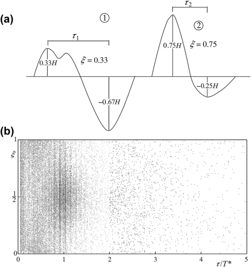
FIGURE 4.4 The waves with a fixed height H generally show a large variety of ξ and τ: two examples are shown in panel
(a). Plotting ξ versus τ; generally we get a wide cloud of points (panel (b)).

Let us suppose to examine a very large time interval

T $T$

, to gather all the waves whose height is in a fixed small interval H, H + dH, and to mark the points representative of these waves in the plane τ-ξ. If H/σ is finite, the marked points would spread over the plane τ-ξ, as we see in Fig. 4.4(b). On the contrary, as H/σ → ∞, we would look at a great concentration: all the points but a negligible share would fall in an open 2-ball with center at

T∗,12 $T^{*}, \frac{1}{2}$

and radius of order (H/σ)⁻¹. In the paper (1989) I obtained a number of these points (see also Sections 9.6–9.10 of my book (2000)). This led to the closed form solution for the asymptotic form of the probability of wave heights in the limit as H/σ → ∞. This is

P(waveheight>H)=K1exp(−H2K2m0),asH/m0−−−√→∞ $P (wave height > H) = K_{1} \exp (- \frac{H^{2}}{K_{2} m_{0}}), as H / \sqrt{m_{0}} \to \infty$

(4.44)

where

K1=(1+ψ¨∗)2ψ¨∗(1+ψ∗)√ $K_{1} = \frac{(1 + {\ddot{ψ}}^{*})}{\sqrt{2 {\ddot{ψ}}^{*} (1 + ψ^{*})}}$

(4.45)

K2=4(1+ψ∗) $K_{2} = 4 (1 + ψ^{*})$

(4.46)

with

ψ∗=∣∣ψ(T∗)ψ(0)∣∣,ψ¨∗=∣∣∣ψ¨(T∗)ψ¨(0)∣∣∣ $ψ^{*} = | \frac{ψ (T^{*})}{ψ (0)} |, {\ddot{ψ}}^{*} = | \frac{\ddot{ψ} (T^{*})}{\ddot{ψ} (0)} |$

(4.47)

With the JONSWAP spectrum, T∗/T_p and ψ∗ are obtained directly from the function ψ(T)/ψ(0) versus T/T_p—Eqn (3.41). As to

ψ¨∗ ${\ddot{ψ}}^{*}$

it is given by

ψ¨∗=∣∣∫∞0E(w)w2cos(2πwT∗Tp)dw∣∣∫∞0E(w)w2dw ${\ddot{ψ}}^{*} = \frac{| \int_{0}^{\infty} E (w) w^{2} \cos (2 π w \frac{T^{*}}{T_{p}}) d w |}{\int_{0}^{\infty} E (w) w^{2} d w}$

(4.48)

The probability Eqn (4.44) is used also in the form

P(α>α¯¯)=K1exp(−α¯¯2K2),asα¯¯→∞ $P (α > \bar{α}) = K_{1} \exp (- \frac{{\bar{α}}^{2}}{K_{2}}), as \bar{α} \to \infty$

(4.49)

where

P(α>α¯¯) $P (α > \bar{α})$

represents the probability that

FIGURE 4.5 Abscissa: the probability of exceedance; ordinate: the quotient between the wave height and the wave height with a very narrow spectrum.
Data points from numerical simulations of stationary Gaussian processes by Forristall (1984).

α=waveheight/σ $α = wave height / σ$

(4.50)

exceeds some fixed threshold

α¯¯ $\bar{α}$

. Equation (4.49) holds as

α¯¯ $\bar{α}$

tends to infinity, that is, as P approaches zero. However, with characteristic spectra of wind seas, it proves to be effective for P smaller than about 0.3, as we may see in Fig. 4.5. This figure shows the ratio

α¯¯(P)/α¯¯R(P)versusP $\bar{α} (P) / {\bar{α}}_{R} (P) versus P$

(4.51)

where

α¯¯ $\bar{α}$

(P) is the value of

α¯¯ $\bar{α}$

that has a given probability P to be exceeded, in a random process with a given spectrum, and α_R(P) is the value of

α¯¯ $\bar{α}$

that has a given probability P to be exceeded in the random process with the very narrow spectrum. The continuous line has been obtained with the asymptotic Eqn (4.49), which gives

α¯¯(P)/α¯¯R(P)=K2ln(K1/P)8ln(1/P)−−−−−−−−−√ $\bar{α} (P) / {\bar{α}}_{R} (P) = \sqrt{K_{2} \frac{\ln (K_{1} / P)}{8 \ln (1 / P)}}$

(4.52)

The data points are from numerical simulations of stationary Gaussian processes by Forristall (1984).

4.6. Field Verification

4.6.1. An Experiment on Wave Periods

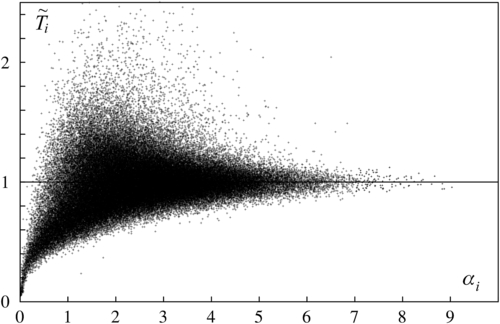
Let us obtain the pairs

αi,T˜i $α_{i}, {\tilde{T}}_{i}$

for i = 1, N with N being the number of waves of a record: α_i is the ratio between the height of the ith wave and the σ of the sea state, and

T˜i ${\tilde{T}}_{i}$

is the ratio between the period of the ith wave and the T_h of the sea state. Let us gather the pairs

αi,T˜i $α_{i}, {\tilde{T}}_{i}$

of a number of records from sea states, generally different from one another, and let us plot these pairs: each pair is represented by one point whose abscissa is α_i and whose ordinate is

T˜i ${\tilde{T}}_{i}$

. We shall obtain a cloud of points like that of Fig. 4.6. From the quasi-determinism (QD) theory, we expect that the rightmost points of the cloud have ordinates close to 1, and this is what typically happens.

4.6.2. The Random Variable β

In view of a verification of the distribution of wave heights in sea states, it is convenient defining a new random variable

β=8(α2K2−lnK1)−−−−−−−−−−−−√ $β = \sqrt{8 (\frac{α^{2}}{K_{2}} - \ln K_{1})}$

(4.53)

β is a monotonic growing function of α, and the inverse function

α=K2(β28+lnK1)−−−−−−−−−−−−−−√ $α = \sqrt{K_{2} (\frac{β^{2}}{8} + \ln K_{1})}$

(4.54)

is a monotonic growing function of β. From Eqn (4.54), it follows that

FIGURE 4.6 Dimensionless wave period versus dimensionless wave height.
Data points from a small scale field experiment of 1990, described in Chapter 9.

P(β>β¯)=P(α>K2(β¯28+lnK1)−−−−−−−−−−−−−−√) $P (β > \bar{β}) = P (α > \sqrt{K_{2} (\frac{{\bar{β}}^{2}}{8} + \ln K_{1})})$

(4.55)

where

β¯ $\bar{β}$

is an arbitrary threshold. Finally, from Eqns (4.49) and (4.55), it follows that

P(β>β¯)=exp(−β¯28),asβ¯→∞ $P (β > \bar{β}) = \exp (- \frac{{\bar{β}}^{2}}{8}), as \bar{β} \to \infty$

(4.56)

If the distribution of α is given by Eqn (4.49), the distribution of β is given by Eqn (4.56), and vice versa. As we may see, the asymptotic distribution of the random variable β does not depend on the spectrum shape.

A clear confirmation of Eqn (4.56) is given by Fig. 4.7, where the data points were obtained from more than six million individual waves from sea states with a large variety of spectra (Boccotti, 2012). We see that the convergence of the data points onto the asymptotic form Eqn (4.56) is very fast: the agreement between data points and asymptotic form being nearly perfect for

β¯>2 $\bar{β} > 2$

The same strict agreement between data points and asymptotic form Eqn (4.56) emerges from a new small-scale field experiment (SSFE) of 2012 on the distribution of wave heights in the space domain (Boccotti, 2013). This represents a strong test of the theory given that the range of values of K₁, K₂ for the waves in the space domain is different from the range of values of K₁, K₂ characteristic of the waves in the time domain. As an example, in the SSFE of 2012:

FIGURE 4.7 P(β>β¯) $P (β > \bar{β})$ from a small-scale field experiment of 2010 on a very large variety of spectra, with a total number of 6,300,000 individual waves.

K₁ (1.1, 2.5) in the space domain → K₁ (1.0, 1.4) in the time domain.

K₂ (4.1, 6.8) in the space domain → K₂ (5.9, 7.6) in the time domain.

4.7. Maximum Expected Wave Height and Crest Height in a Sea State of Given Characteristics

4.7.1. The Maximum Expected Wave Height

Let us consider N consecutive waves of a sea state of given significant height. The probability that the largest wave height of this set of N waves is smaller than a given threshold H is equal to the probability that all the N wave heights are smaller than H, that is,

P(Hmax<H)=[1−P(waveheight>H)]N $P (H_{\max} < H) = {[1 - P (wave height > H)]}^{N}$

(4.57)

which implies

P(Hmax>H)=1−[1−P(waveheight>H)]N $P (H_{\max} > H) = 1 - {[1 - P (wave height > H)]}^{N}$

(4.58)

Equations (4.57) and (4.58) are based on the assumption that the wave heights are stochastically independent of one another. Given that this assumption is not fully satisfied, Eqn (4.58) is slightly conservative, in that it slightly overpredicts the probability of exceedance of H_max (see Section 5.10.1 of Boccotti, 2000).

The mean value of a positive random variable V, like H_max, is related to the probability of exceedance P(V > x) by

V¯¯¯=∫∞0P(V>x)dx $\bar{V} = \int_{0}^{\infty} P (V > x) d x$

(4.59)

Hence, in the special case that V = H_max, we have

Hmax¯¯¯¯¯¯¯=∫∞0P(Hmax>H)dH $\bar{H_{\max}} = \int_{0}^{\infty} P (H_{\max} > H) d H$

(4.60)

In order to understand the meaning of

Hmax¯¯¯¯¯¯¯ $\bar{H_{\max}}$

, let us imagine taking n sets each of N consecutive waves from a sea state. The first set will have a maximum wave height H_max1, the second set will have a maximum wave height H_max2 generally different from H_max1, and so on as far as the nth set whose maximum wave height will be H_maxn.

Hmax¯¯¯¯¯¯¯ $\bar{H_{\max}}$

represents the average of H_max1, H_max2, etc. Equations (4.44), (4.58), and (4.60) yield

Hmax¯¯¯¯¯¯¯=∫0∞1−[1−K1exp(−H2K2m0)]NdH $\bar{H_{\max}} = \int_{0}^{\infty} 1 - {[1 - K_{1} \exp (- \frac{H^{2}}{K_{2} m_{0}})]}^{N} d H$

(4.61)

The use of the asymptotic form Eqn (4.44) of P(wave height > H) is justified because the integrand in Eqn (4.60) gets appreciably different from 1 for H/σ definitely greater than 4 wherein the asymptotic form proves to be fully efficient.

4.7.2. Maximum Expected Crest Height

The reasoning done for

Hmax¯¯¯¯¯¯¯ $\bar{H_{\max}}$

may be repeated for obtaining

bmax¯¯¯¯¯¯ $\bar{b_{\max}}$

, the maximum expected height of a wave crest. We have

bmax¯¯¯¯¯¯=∫0∞P(bmax>b)db $\bar{b_{max}} = \int_{0}^{\infty} P (b_{\max} > b) d b$

(4.62)

that is,

bmax¯¯¯¯¯¯=∫0∞1−[1−P(C>b)]Ndb $\bar{b_{\max}} = \int_{0}^{\infty} 1 - {[1 - P (C > b)]}^{N} d b$

(4.63)

and, with the asymptotic form Eqn (4.32) of P(C > b):

bmax¯¯¯¯¯¯=∫0∞1−[1−exp(−b22m0)]Ndb $\bar{b_{\max}} = \int_{0}^{\infty} 1 - {[1 - \exp (- \frac{b^{2}}{2 m_{0}})]}^{N} d b$

(4.64)

bmax¯¯¯¯¯¯ $\bar{b_{\max}}$

proves to be greater than

Hmax¯¯¯¯¯¯¯/2 $\bar{H_{\max}} / 2$

4.8. FORTRAN Programs for the Maximum Expected Wave in a Sea State of Given Characteristics

The characteristics of a sea state are H_s, duration, and spectrum shape. Here, we assume to know these characteristics and aim to estimate height and period of the maximum expected wave. The following FORTRAN programs serve for this aim.

4.8.1. A Program for the Basic Parameters on Deep Water

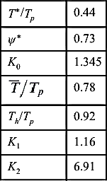
Program SUMMARY calculates T∗/T_p and ψ∗ (Eqn (3.41)), K₀ (Eqn (3.46)), T_m/T_p (Eqn (4.39)), T_h/T_p (Eqn (4.43)),

ψ¨∗ ${\ddot{ψ}}^{*}$

(Eqn (4.48)), K₁ (Eqn (4.45)), and K₂ (Eqn (4.46)) with the JONSWAP spectrum. The equations of these parameters have been obtained throughout Chapters 3 and 4; hence, the title SUMMARY of the program. With the JONSWAP spectrum these parameters depend only on function

E(w) $E (w)$

defined by Eqn (3.42), which calls for two shape parameters χ₁, χ₂.

    PROGRAM SUMMARY
    DIMENSION EW(500),WV(500)
    DIMENSION TAUV(200),ETADET(200),TZU(5)
    PG=3.141592
    DPG=2.∗PG
    WRITE(6,∗)'chi1,chi2'
    READ(5,∗)CHI1,CHI2
    C1=ALOG(CHI1)
    C2=2∗CHI2∗CHI2
    WIN=0.5
    WMAX=5

c calculation of E(w) -Eqn (3.42)-

    DW=0.02
    W=WIN-DW/2
    I=0
90   W=W+DW
    IF(W.GT.WMAX)GO TO 91
    I=I+1
    WM1=W-1
    W2=W∗W
    W4=W2∗W2
    W5=W4∗W
    ARG3=WM1∗WM1/C2
    E3=EXP(-ARG3)
    ARG2=C1∗E3
    E2=EXP(ARG2)
    ARG1=1.25/W4
    E1=EXP(-ARG1)
 
c values of w and E(w) stored on memory
    WV(I)=W
    EW(I)=E1∗E2/W5
    GO TO 90
91   CONTINUE
    IMAX=I

c calculation of T∗/Tp and psi∗
    PSIMIN=0
    DTAU=0.01
    TAU=-DTAU
70   TAU=TAU+DTAU
c Loop 70 tau (=T/Tp) from 0 to 1
    IF(TAU.GT.1) GO TO 71

c SOMT integral, numerator of the RHS of Eqn (3.41)

c SOM0 integral, denominator of the RHS of Eqn (3.41)

    SOMT=0
    SOM0=0
    DO 75 I=1,IMAX
c Loop 75 over the stored values of w and E(w)
    W=WV(I)
    COSA=COS(DPG∗W∗TAU)
    SOMT=SOMT+EW(I)∗COSA∗DW
    SOM0=SOM0+EW(I)∗DW
75   CONTINUE
    PSI=SOMT/SOM0
c PSI=psi(T)/psi(0)
    IF(PSI.LT.PSIMIN)THEN
    PSIMIN=PSI
    TAUMI=TAU
    ENDIF
    GO TO 70
71   CONTINUE
    TASTP=TAUMI
    PSIAS=ABS(PSIMIN)
c TASTP=T∗/Tp
c PSIAS=psi∗

c calculation of K0 - Eqn (3.46)-

    SOM0=0

c SOM0 integral on the RHS of Eqn (3.46)

    DO I=1,IMAX
    SOM0=SOM0+EW(I)∗DW
    ENDDO
    RK0=1./SOM0∗∗0.25

c calculation of Tm/Tp - Eqn (4.39) -

c SOM0 integral, numerator of the RHS of Eqn (4.39)

c SOM2 integral, denominator of the RHS of Eqn (4.39)

 
    SOM0=0
    SOM2=0
    DO I=1,IMAX
    W=WV(I)

    .SOM0=SOM0+EW(I)∗DW
    SOM2=SOM2+EW(I)∗W∗W∗DW
    ENDDO
    TMTP=SQRT(SOM0/SOM2)
 
c TMTP=Tm/Tp
c calculation of Th/Tp
    DTAU=0.01
    TAUI=-0.5
    TAUF=1
    TAU=TAUI-DTAU
    J=0
80   TAU=TAU+DTAU
c Loop 80: TAU=T/Tp from -0.5 to 1
    IF(TAU.GT.TAUF)GO TO 81
    J=J+1

c SOM1 integral, numerator of the RHS of Eqn (4.43)

c SOM2 integral, denominator of the RHS of Eqn (4.43)

    SOM1=0
    SOM2=0
    DO I=1,IMAX
    W=WV(I)
    ARG1=DPG∗W∗TAU
    ARG2=DPG∗W∗(TAU-TASTP)
    ARG3=DPG∗W∗TASTP
    SOM1=SOM1+EW(I)∗(COS(ARG1)-COS(ARG2))∗DW
    SOM2=SOM2+EW(I)∗(1-COS(ARG3))∗DW
    ENDDO
    ETADET(J)=0.5∗SOM1/SOM2
    TAUV(J)=TAU

c ETADET(J) = eta deterministic(tau)/H - Eqn (4.43) -

c TAUV(J)=T/Tp
 
    GO TO 80
81   CONTINUE
    JMAX=J
 
    NZU=0
    DO 65 J=2,JMAX

c Loop 65 over the stored values of eta deterministic(tau)/H - Eqn (4.43) -2

    TAU=TAUV(J)
    IF(ETADET(J).GE.0.AND.ETADET(J-1).LT.0)THEN
    NZU=NZU+1
    E1=-ETADET(J-1)
    E2=ETADET(J)
    TZU(NZU)=TAU-DTAU+DTAU∗E1/(E1+E2)

    .ENDIF
65   CONTINUE
    THTP=TZU(2)-TZU(1)
c THTP=Th/Tp

c calculation of psi..∗ - Eqn (4.48) -

c SOM1 integral, numerator of the RHS of Eqn (4.48)

c SOM2 integral, denominator of the RHS of Eqn (4.48)

    SOM1=0
    SOM2=0
    DO I=1,IMAX
    W=WV(I)
    W2=W∗W
    ARG=DPG∗W∗TASTP
    COSA=COS(ARG)
    SOM1=SOM1+EW(I)∗W2∗COSA∗DW
    SOM2=SOM2+EW(I)∗W2∗DW
    ENDDO
    PSIS=ABS(SOM1/SOM2)
c PSIS=psi..∗

c calculation of K1 -Eqn (4.45)-

    RNUM=1+PSIS
    RDEN=SQRT(2.∗PSIS∗(1.+PSIAS))
    RK1=RNUM/RDEN

c calculation of K2 -Eqn (4.46)-

    RK2=4.∗(1.+PSIAS)
 
    WRITE(6,1001)TASTP
    WRITE(6,1002)PSIAS
    WRITE(6,1003)RK0
    WRITE(6,1004)TMTP
    WRITE(6,1005)THTP
    WRITE(6,1006)RK1
    WRITE(6,1007)RK2
1001  FORMAT(2X,'T∗/Tp ',f7.2)
1002  FORMAT(2X,'psi∗ ',f7.2)
1003  FORMAT(2X,'K0 ',f7.3)
1004  FORMAT(2X,'Tm/Tp ',f7.2)
1005  FORMAT(2X,'Th/Tp ',f7.2)
1006  FORMAT(2X,'K1 ',f7.2)
1007  FORMAT(2X,'K2 ',f7.2)
    END

In this program, TAU is the ratio T/T_p. The function of TAU on the RHS of Eqn (4.43) is calculated from TAUI = −0.5 to TAUF = 1 with a step DTAU = 0.01 and is stored on the vector ETADET. Then the program searches the two zero up-crossings of this function, in the domain (TAUI, TAUF). The TAU of the first zero up-crossing is TZU(1), and the TAU of the second zero up-crossing is TZU(2)—see Fig. 4.3. T_h/T_p is equal to the interval (TZU(2) − TZU(1)). With the mean JONSWAP spectrum (χ₁ = 3.3, χ₂ = 0.08), the program gives the values of Table 4.1.

Table 4.1

Values of Some Basic Parameters in Sea States with the Mean JONSWAP Spectrum

T^∗/T_p	0.44
ψ^∗	0.73
K₀	1.345
T¯¯¯/Tp $\bar{T} / T_{p}$	0.78
T_h/T_p	0.92
K₁	1.16
K₂	6.91

4.8.2. A Program for the Basic Parameters on a Finite Water Depth, Using the Shape of the TMA Spectrum

A program for finite water, which we shall call SUMM1, may be obtained with the following changes from SUMMARY:

1. d and T_p must be supplied as inputs (hence the part of the program concerning K₀ may be canceled), and T_p may be obtained running SUMMARY for deep water;

2. the dimensionless spectrum

E(w) $E (w)$

must be multiplied by the transformation function TFU (see Section 3.4.6); specifically the line

   EW(I)=E1∗E2/W5

must be changed into

   EW(I)=TFU(W,DLP0)∗E1∗E2/W5

where DLP0 is the ratio d/L_p0.

The transformation function is listed here:

   FUNCTION TFU(w,DLP0)
   PG=3.141592
   DPG=2.∗PG

c calculation of the dimensionless wave number - Eqn (3.51)-

   W2=W∗W
   DX=1
   X=0
110  X=X+DX
   F=X∗TANH(DPG∗X∗DLP0)
   IF(F.LT.W2)GO TO 110
   X=X-DX
   DX=DX/10.
   IF(DX.GT.2.E4)GO TO 110
   RKW=X
c RKW=kw

c calculation of TFU: function on the RHS of Eqn (3.52) divided by E0(w)

   ARG=4.∗PG∗RKW∗DLP0
   IF(ARG.LT.30.)THEN
   SI2=SINH(ARG)
   DEN=SI2+ARG
   RMOL=SI2/DEN
   ARG=ARG/2
   TA=TANH(ARG)
   TFU=TA∗TA∗RMOL
   ELSE
   TFU=1
   ENDIF
   RETURN
   END

4.8.3. A Program for the Maximum Expected Wave Height

The third program is HMAX. It calculates

Hmax¯¯¯¯¯¯¯ $\bar{H_{\max}}$

in a sequence of N waves of given H_s and given spectrum:

   PROGRAM HMAX
   DOUBLE PRECISION UPH,PC,PDBLE
   CHARACTER∗64 NOMEC
   NOMEC='PROHMAX'
   OPEN(UNIT=66,FILE=NOMEC)
   WRITE(6,∗)'Hs,N'
   READ(5,∗)HS,N
   WRITE(6,∗)'K1,K2'
   READ(5,∗)RK1,RK2
   SIG=HS/4.
   RM0=SIG∗SIG
   DH=0.10
   HMA=0
c HMA value of the integral to be executed in the loop 90

H=-DH/2.

  .90H=H+DH

c Loop 90: integral with respect to H on the RHS of Eqn (4.61)

   IF(H.GT.3.∗HS)GO TO 91
   ARG=H∗H/(RK2∗RM0)
   EE=EXP(-ARG)
   PH=RK1∗EE
   UPH=1.-DBLE(PH)
   PC=UPH∗∗N
   PDBLE=1.-PC
   P=PDBLE
c P=P(Hmax>H)
   WRITE(66,1010)H,P
1010 FORMAT(2X,F7.2,2X,E12.4)
   HMA=HMA+P∗DH
   GO TO 90
91   CONTINUE
   WRITE(6,1000)HMA
1000 FORMAT(2X,'Hmax ',f7.2)
   WRITE(6,∗)'read file prohmax'
   END

4.8.4. Worked Example

Deep water sea state: H_s = 8 m, duration = 5 h, spectrum: mean JONSWAP with A = 0.01.

1. Calculation of T_p by means of Eqn (3.47):

Tp=1.3450.01√4π8/9.8−−−−√=12.1s $T_{p} = \frac{1.345}{\sqrt[4]{0.01}} π \sqrt{8 / 9.8} = 12.1 s$

2. Calculation of T_m:

Tm=0.78Tp=9.4s $T_{m} = 0.78 T_{p} = 9.4 s$

3. Calculation of the number of waves in the sea state:

N=duration/Tm=5⋅3600/9.4=1915 $N = duration / T_{m} = 5 \cdot 3600 / 9.4 = 1915$

4. The run of program HMAX with input data H_s = 8 m, N = 1915, K₁ = 1.16, K₂ = 6.91 gives

Hmax¯¯¯¯¯¯¯=15.1m $\bar{H_{\max}} = 15.1 m$

5. Calculation of T_h:

Th=0.92Tp=11.1s $T_{h} = 0.92 T_{p} = 11.1 s$

FIGURE 4.8 Worked example of Section 4.8.4:
Probability P (ordinate) that the maximum wave height in a given sea state exceeds a given threshold H (abscissa). The maximum expected wave height in the sea state is the integral of this function on (0,∞).

Conclusion: the maximum expected wave in the given sea state has a height of 15.1 m and a period of 11.1 s. Figure 4.8 shows the probability P(H_max > H), which is written by program HMAX on file PROHMAX (H: first column; P: second column).

4.9. Conclusion

I introduced Eqns (4.42) and (4.44) (or Eqn (4.49)), respectively, in the papers (1984) and (1989), as corollaries of the QD theory. Various comparisons of the asymptotic distribution (Eqn (4.49)) with oceanic data (Tayfun and Fedele, 2007; Casas–Prat and Holthuijsen, 2010) tend to support the effectiveness of this distribution, also under the effects of second-order corrections. The effects of third-order corrections may be of some relevance in wind seas, wherein the spectrum exhibits significant variability in space and/or time. These effects were dealt with under the narrowband assumption, by Tayfun and Lo (1990), Mori and Janssen (2006), Tayfun and Fedele (2007), Cherneva et al. (2009, 2013), Fedele et al. (2010). Resorting to Gram–Charlier series expansions was convenient, and the Gram–Charlier series approximation for the distribution of the wave heights (under narrowband assumption) proved to be (Tayfun and Fedele, 2007)

P(α>α¯¯)=exp(−α¯¯28)[1+Λ1024α¯¯2(α¯¯2−16)] $P (α > \bar{α}) = \exp (- \frac{{\bar{α}}^{2}}{8}) [1 + \frac{Λ}{1024} {\bar{α}}^{2} ({\bar{α}}^{2} - 16)]$

(4.65)

where

Λ=λ40+2λ22+λ04 $Λ = λ_{40} + 2 λ_{22} + λ_{04}$

(4.66)

and

λ40=⟨(η(t)/σ)4⟩−3 $λ_{40} = 〈 {(η (t) / σ)}^{4} 〉 - 3$

(4.67)

λ22=⟨(η(t)/σ)2(ηˆ(t)/σ)2⟩−1 $λ_{22} = 〈 {(η (t) / σ)}^{2} {(\hat{η} (t) / σ)}^{2} 〉 - 1$

(4.68)

λ04=⟨(ηˆ(t)/σ)4⟩−3 $λ_{04} = 〈 {(\hat{η} (t) / σ)}^{4} 〉 - 3$

(4.69)

with

ηˆ(t) $\hat{η} (t)$

being the Hilbert transform of η(t). The fourth-order cumulants λ₄₀, λ₂₂, and λ₀₄ are indexes of the differences between η(t) and a stationary Gaussian process for which these cumulants are equal to zero. Then Alkhalidi and Tayfun (2013) suggested to generalize Eqn (4.49) into the form

P(α>α¯¯)=K1exp(−α¯¯2K2)[1+Λ16(α¯¯2K2)(α¯¯2K2−2)] $P (α > \bar{α}) = K_{1} \exp (- \frac{{\bar{α}}^{2}}{K_{2}}) [1 + \frac{Λ}{16} (\frac{{\bar{α}}^{2}}{K_{2}}) (\frac{{\bar{α}}^{2}}{K_{2}} - 2)]$

This form proved to be able to fit rather well even artificially created waveflume conditions with rather large value of

Λ $Λ$

due to fully developed third-order free–wave interactions.

..................Content has been hidden....................

You can't read the all page of ebook, please click here login for view all page.

Table of Contents for Chapter 4. Wave Statistics in Sea States

Create new playlist

Sign In

Sign Up

Abstract

Keywords

4.1. Surface Elevation as a Stationary Gaussian Process

4.1.1. The Probability of the Surface Elevation

4.1.2. Proof Relevant to Any Given Realization

4.1.3. Proof Relevant to the Ensemble at a Fixed Time Instant

4.2. Joint Probability of Surface Elevation

4.3. Rice's Problem (1958)

4.4. Corollaries of Rice's Problem

4.4.1. Probability of Crest Height and Wave Height

4.4.2. The Mean Wave Period

4.5. Consequences of the QD Theory onto Wave Statistics

4.5.1. Period Th of a Very Large Wave

4.5.2. The Wave Height Probability under General Bandwidth Assumptions

4.6. Field Verification

4.6.1. An Experiment on Wave Periods

4.6.2. The Random Variable β

4.7. Maximum Expected Wave Height and Crest Height in a Sea State of Given Characteristics

4.7.1. The Maximum Expected Wave Height

4.7.2. Maximum Expected Crest Height

4.8. FORTRAN Programs for the Maximum Expected Wave in a Sea State of Given Characteristics

4.8.1. A Program for the Basic Parameters on Deep Water

4.8.2. A Program for the Basic Parameters on a Finite Water Depth, Using the Shape of the TMA Spectrum

4.8.3. A Program for the Maximum Expected Wave Height

4.8.4. Worked Example

4.9. Conclusion

Table of Contents for
Chapter 4. Wave Statistics in Sea States

4.5.1. Period T_h of a Very Large Wave