Search in book...
Toggle Font Controls
Create new playlist

Name your new playlist

Playlist description (optional)
Sign In

Email address

Password

Forgot Password?

or

Continue with Facebook

Continue with Google
Sign Up

Full Name

Email address

Confirm Email Address

Password

or

Continue with Facebook

Continue with Google

Chapter 2

Wave Transformation near Coasts

Abstract

A first part of the chapter deals with wave refraction before a coast. Effects on wave heights and wave directions are dealt with analytically for the case of straight contour lines, and the numerical approach is explained in detail for arbitrary contour lines. The second part of the chapter is devoted to the problem of shoaling and set-down (or set-up) of waves on a current. The way to calculate the current effect on wavelength and wave height is shown. A FORTRAN program is given and applied to a worked example of calculation of the Froude–Krylov force on a submerged tunnel across a strait with waves and current.

Keywords

Coast; Froude–Krylov force; Strait; Submerged tunnel; Wave-current; Wavelength; Wave height; Wave orthogonal; Wave refraction

2.1. Refraction with Straight Contour Lines

With reference to Fig. 2.1, s is the local direction of wave advance at a point P on water depth, d, and α is the angle between the wave direction and x-axis. We assume that the seabed is gently sloped so that in a neighborhood of point P, the horizontal particle velocity is

$v_{s} (s, z, t) = g \frac{H}{2} ω^{- 1} k \frac{\cosh [k (d + z)]}{\cosh (k d)} \cos (k s - ω t)$ $v_{s} (s, z, t) = g \frac{H}{2} ω^{- 1} k \frac{\cosh [k (d + z)]}{\cosh (k d)} \cos (k s - ω t)$

(2.1)

FIGURE 2.1 Reference scheme: waves approaching a coast.

The x,y component of the radiation stress tensor, that is, the x-component of the mean flux of linear momentum, per unit length, through a y-orthogonal plane is

$R_{y x} = 〈 \int_{- d}^{η} ρ v_{s}^{2} \sin α \cos α d z 〉$ $R_{y x} = 〈 \int_{- d}^{η} ρ v_{s}^{2} \sin α \cos α d z 〉$

(2.2)

Here we may proceed like we have done for Φ in Section 1.9. That is, we neglect the terms of order smaller than H², which enables us to pass

$from \int_{- d}^{η} to \int_{- d}^{0}$ $from \int_{- d}^{η} to \int_{- d}^{0}$

then we invert the order average with respect to time t—integral with respect to z, and we can arrive at

$R_{x y} = R_{y x} = \frac{1}{16} ρ g H^{2} [1 + \frac{2 k d}{\sinh (2 k d)}] \sin α \cos α$ $R_{x y} = R_{y x} = \frac{1}{16} ρ g H^{2} [1 + \frac{2 k d}{\sinh (2 k d)}] \sin α \cos α$

(2.3)

Let us consider the control volume (CV) of Fig. 2.2 before a coast. Because of the x-parallel contour lines, the mean characteristics of the wave motion do not change with x and change only with y. Therefore, the energy equation and the x-component of the linear momentum equation when applied to the CV of Fig. 2.2 give

$Φ (y_{2}) \sin α_{2} = Φ (y_{1}) \sin α_{1}$ $Φ (y_{2}) \sin α_{2} = Φ (y_{1}) \sin α_{1}$

(2.4)

$R_{y x} (y_{2}) = R_{y x} (y_{1})$ $R_{y x} (y_{2}) = R_{y x} (y_{1})$

(2.5)

If y₁ is on deep water and y₂ is on water depth, d, these two equations yield

$H^{2} \tanh (k d) [1 + \frac{2 k d}{\sinh (2 k d)}] \sin α = H_{0}^{2} \sin α_{0}$ $H^{2} \tanh (k d) [1 + \frac{2 k d}{\sinh (2 k d)}] \sin α = H_{0}^{2} \sin α_{0}$

(2.6)

FIGURE 2.2 The control volume extending from water depth d₁ to water depth d₂, with straight contour lines.

$H^{2} [1 + \frac{2 k d}{s i n h (2 k d)}] s i n α \cos α = H_{0}^{2} s i n α_{0} \cos α_{0}$ $H^{2} [1 + \frac{2 k d}{s i n h (2 k d)}] s i n α \cos α = H_{0}^{2} s i n α_{0} \cos α_{0}$

(2.7)

where use has been made of Eqn (1.97) of Φ and Eqn (2.3) of R_yx.

From (Eqns (2.6) and (2.7)) we obtain

$\cos α = \cos α_{0} \tanh (k d) = \cos α_{0} c / c_{0}$ $\cos α = \cos α_{0} \tanh (k d) = \cos α_{0} c / c_{0}$

(2.8)

which enables us to obtain angle α on water depth, d, once angle α₀ on deep water is known.

Referring to the basic case in which the wave travels landward, angles α₀ and α range between 0 and π, and thus

$s i n α_{0} = \sqrt{1 - \cos^{2} α_{0}}$ $s i n α_{0} = \sqrt{1 - \cos^{2} α_{0}}$

(2.9)

$s i n α = \sqrt{1 - \tanh^{2} (k d) \cos^{2} α_{0}}$ $s i n α = \sqrt{1 - \tanh^{2} (k d) \cos^{2} α_{0}}$

(2.10)

At this stage, with cos α and sin α being known, we can operate on either (Eqn (2.6)) or (Eqn (2.7)) to obtain also H. The result is

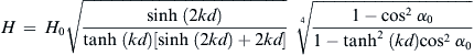$H = H_{0} \sqrt{\frac{\sinh (2 k d)}{\tanh (k d) [\sinh (2 k d) + 2 k d]}} \sqrt[4]{\frac{1 - \cos^{2} α_{0}}{1 - \tanh^{2} (k d) \cos^{2} α_{0}}}$ $H = H_{0} \sqrt{\frac{\sinh (2 k d)}{\tanh (k d) [\sinh (2 k d) + 2 k d]}} \sqrt[4]{\frac{1 - \cos^{2} α_{0}}{1 - \tanh^{2} (k d) \cos^{2} α_{0}}}$

(2.11)

This equation enables us to get wave height H on water depth d, once height H₀ and angle α₀ on deep water are known. The ratio H/H₀ for α₀ = 90° is the shoaling coefficient (C_s).

Figure 2.3 shows the ratio H/H₀ as a function of d/L₀ for some given value of α₀. (Note Eqn (2.11) gives H/H₀ as a function of kd, whereas Fig. 2.3 shows H/H₀ as a function of d/L₀. This is possible because kd is a function of d/L₀. Indeed from (Eqn (1.24)), it follows that

$\frac{d}{L_{0}} = \frac{d}{L} \tanh (2 π \frac{d}{L})$ $\frac{d}{L_{0}} = \frac{d}{L} \tanh (2 π \frac{d}{L})$

(2.12)

which implies that a unique value of kd = 2πd/L exists for any given value of d/L₀.) As d/L₀ approaches zero, H/H₀ tends to infinity. Of course, this growth of wave height is interrupted by wave breaking.

2.2. Refraction with Arbitrary Contour Lines

2.2.1. Wave Orthogonals

In the previous section, we solved the problem of the control volume extending from deep to shallow water for the basic case of straight contour lines. Here, we deal with the same problem for the case of arbitrary contour lines. To this end, it is convenient to preliminarily solve the refraction problem.

FIGURE 2.3 Variation of the wave height with the water depth for given wave direction on deep water. (Obtained by means of Eqn (2.11).)

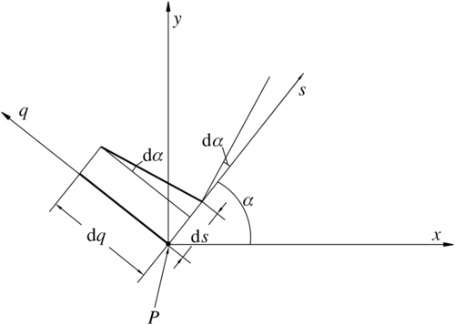
Let us fix a point P in the horizontal plane, and let us define the natural coordinates: s with the local wave direction and q orthogonal to s. The inclination of a small stretch dq of wave front varies in a small time interval dt of

$d α = \frac{c d t - (c + \frac{\partial c}{\partial q} d q) d t}{d q} = - \frac{\partial c}{\partial q} d t$ $d α = \frac{c d t - (c + \frac{\partial c}{\partial q} d q) d t}{d q} = - \frac{\partial c}{\partial q} d t$

(2.13)

where α and c denote, respectively, the angle of the wave front and the propagation speed at point P (see Fig. 2.4). Since

$d s = c d t$ $d s = c d t$

(2.14)

(Eqn (2.13)) may by rewritten as

$\frac{d α}{d s} = - \frac{1}{c} \frac{\partial c}{\partial q}$ $\frac{d α}{d s} = - \frac{1}{c} \frac{\partial c}{\partial q}$

(2.15)

Here, it is convenient to express

\partial c / \partial q

$\partial c / \partial q$

in terms of the derivatives

\partial c / \partial x

$\partial c / \partial x$

and

\partial c / \partial y

$\partial c / \partial y$

(x and y being as usual the fixed axes). Since

$\frac{\partial c}{\partial q} d q = \frac{\partial c}{\partial x} (- d q s i n α) + \frac{\partial c}{\partial y} d q \cos α$ $\frac{\partial c}{\partial q} d q = \frac{\partial c}{\partial x} (- d q s i n α) + \frac{\partial c}{\partial y} d q \cos α$

(2.16)

it follows that

$\frac{d α}{d s} = \frac{1}{c} (\frac{\partial c}{\partial x} \sin α - \frac{\partial c}{\partial y} \cos α)$ $\frac{d α}{d s} = \frac{1}{c} (\frac{\partial c}{\partial x} \sin α - \frac{\partial c}{\partial y} \cos α)$

(2.17)

FIGURE 2.4 Refraction: the short stretch dq of wave front, covering the distance ds, rotates through dα.

Applying the chain rule, Eqn (2.17) may be rewritten in the form

$\frac{d α}{d s} = \frac{1}{c} (\frac{d c}{d d} \frac{\partial d}{\partial x} \sin α - \frac{d c}{d d} \frac{\partial d}{\partial y} \cos α)$ $\frac{d α}{d s} = \frac{1}{c} (\frac{d c}{d d} \frac{\partial d}{\partial x} \sin α - \frac{d c}{d d} \frac{\partial d}{\partial y} \cos α)$

(2.18)

Hence, obtaining the formula of dc/dd from (Eqn (1.24)) of L, we arrive at

$\frac{d α}{d s} = \frac{2 k}{\sinh (2 k d) + 2 k d} (\frac{\partial d}{\partial x} \sin α - \frac{\partial d}{\partial y} \cos α)$ $\frac{d α}{d s} = \frac{2 k}{\sinh (2 k d) + 2 k d} (\frac{\partial d}{\partial x} \sin α - \frac{\partial d}{\partial y} \cos α)$

(2.19)

This form of dα/ds is convenient for obtaining a wave orthogonal; that is, a curve whose tangent vector gives the local wave direction. Given angle α₀ and a point x₀,y₀ of the orthogonal on deep water, this orthogonal is calculated with finite increments Δs through

$α (s + Δ s) = α (s) + \frac{d α}{d s} Δ s$ $α (s + Δ s) = α (s) + \frac{d α}{d s} Δ s$

(2.20)

$x (s + Δ s) = x (s) + \cos α Δ s - \frac{1}{2} \sin α \frac{d α}{d s} Δ s^{2}$ $x (s + Δ s) = x (s) + \cos α Δ s - \frac{1}{2} \sin α \frac{d α}{d s} Δ s^{2}$

(2.21)

$y (s + Δ s) = y (s) + \sin α Δ s + \frac{1}{2} \cos α \frac{d α}{d s} Δ s^{2}$ $y (s + Δ s) = y (s) + \sin α Δ s + \frac{1}{2} \cos α \frac{d α}{d s} Δ s^{2}$

(2.22)

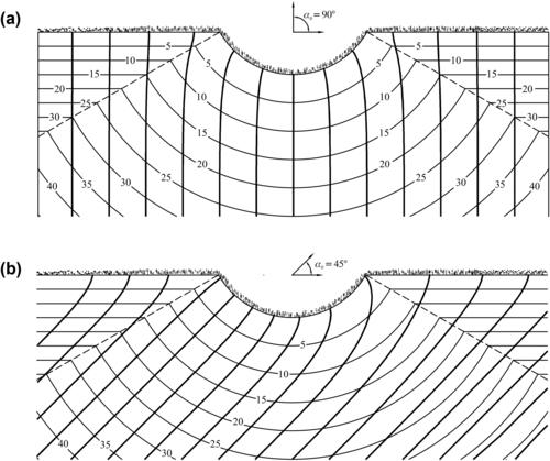
Of course, the wave orthogonal depends on the wave period. As an example, Fig. 2.5 shows some wave orthogonals before a promontory, for two distinct values of angle α₀, and the same wave period.

2.2.2. Effects on the Wave Height

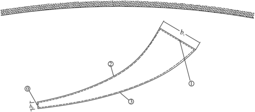
Let us consider a CV whose horizontal section is bounded by two adjacent wave orthogonals (2 and 3 in Fig. 2.6) and two short stretches of wave front (0 and 1 in Fig. 2.6). There is no energy flux through the two orthogonals. Hence, the mean energy flux through the stretch of wave front 0 on deep water must equal the mean energy flux through the stretch of wave front 1 on given water depth d. With Eqn (1.97) of the mean energy flux per unit length, we obtain

FIGURE 2.5 Two sets of wave orthogonals ((a) and (b)) for two distinct wave directions on deep water, and the same wave period (T = 10 s). (Obtained by means of Eqns (2.19)–(2.22).)

$\frac{1}{8} ρ g H_{0}^{2} c_{0} \frac{1}{2} b_{0} = \frac{1}{8} ρ g H^{2} c \frac{1}{2} [1 + \frac{2 k d}{\sinh (2 k d)}] b_{1}$ $\frac{1}{8} ρ g H_{0}^{2} c_{0} \frac{1}{2} b_{0} = \frac{1}{8} ρ g H^{2} c \frac{1}{2} [1 + \frac{2 k d}{\sinh (2 k d)}] b_{1}$

(2.23)

which is reduced to

$H = H_{0} \sqrt{\frac{\sinh (2 k d)}{\tanh (k d) [\sinh (2 k d) + 2 k d]}} \sqrt{\frac{b_{0}}{b_{1}}}$ $H = H_{0} \sqrt{\frac{\sinh (2 k d)}{\tanh (k d) [\sinh (2 k d) + 2 k d]}} \sqrt{\frac{b_{0}}{b_{1}}}$

(2.24)

where d, H, and k are water depth, wave height, and wave number at section ①, and H₀ is the wave height at section ⓪ on deep water. Clearly, this result requires b₁ to be small enough and for the wave height to be nearly constant on the stretch of wave front.

FIGURE 2.6 A control volume from deep to shallow water bounded by two wave orthogonals and two short stretches of wave front.

2.3. Wave–Current Interaction in Some Straits

2.3.1. Current Only

Let us consider a marine strait. To fix our ideas, we may think of the Straits of Messina. Along the longitudinal axis, the water depth reduces to a minimum. In particular, in the Straits of Messina, the water depth is at a minimum (nearly 100 m) somewhat northerly of Messina. Often, some currents take place where the strait has its lowest depth. These currents in the Straits of Messina are due to the flow from the Ionian Sea to the Tyrrhenian Sea and vice versa.

Let us think of a strait as a straight channel of constant width, with a minimum water depth at y = 0 and with water depth tending to infinity as y → ±∞. As in the problem of shoaling-refraction, let us assume the bottom slope to approach zero.

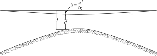
Let us analyze first the case of a current without waves, with a discharge Q per unit length. Referring to Fig. 2.7, we call

S	the difference between the still water level and the actual water level;
d	the depth of the still water;
$\tilde{d} \equiv d - S$ $\tilde{d} \equiv d - S$	the water depth; and
$u = Q / \tilde{d}$ $u = Q / \tilde{d}$	the velocity of the current.

Under ideal flow assumptions, the Bernoulli equation implies

$S = \frac{u^{2}}{2 g}$ $S = \frac{u^{2}}{2 g}$

(2.25)

As a consequence, u, d, and Q are related to each other by

$u = \frac{Q}{d - u^{2} / 2 g}$ $u = \frac{Q}{d - u^{2} / 2 g}$

(2.26)

which may be rewritten in the form

$\frac{u d}{Q} = 1 + {(\frac{Q}{Q^{*}})}^{2} {(\frac{u d}{Q})}^{3}$ $\frac{u d}{Q} = 1 + {(\frac{Q}{Q^{*}})}^{2} {(\frac{u d}{Q})}^{3}$

(2.27)

with

$Q^{*} \equiv \sqrt{2 g d} d$ $Q^{*} \equiv \sqrt{2 g d} d$

(2.28)

Equality (Eqn (2.27)) admits two positive solutions for ud/Q, provided that

$| Q | < Q_{\max} = \frac{2}{3 \sqrt{3}} Q^{*}$ $| Q | < Q_{\max} = \frac{2}{3 \sqrt{3}} Q^{*}$

(2.29)

The lowest of these two solutions is the right one. The second solution yields d − S → 0 as Q approaches zero, and hence must be discarded.

2.3.2. Current + Waves: The Wavelength

If we multiply by d both sides of (Eqn (1.53)) and use definition (Eqn (1.26)) of L₀, we may rewrite (Eqn (1.53)) in the form

$\frac{d}{L_{c}} \tanh (2 π \frac{d}{L_{c}}) = a {(\frac{d}{L_{c}} - b)}^{2}$ $\frac{d}{L_{c}} \tanh (2 π \frac{d}{L_{c}}) = a {(\frac{d}{L_{c}} - b)}^{2}$

(2.30)

where L_c denotes wavelength on current:

FIGURE 2.7 Reference scheme for a steady current on a channel of varying depth.
The bottom slope is assumed to approach zero.

$L_{c} \equiv 2 π / k_{c}$ $L_{c} \equiv 2 π / k_{c}$

(2.31)

and where

$a \equiv \frac{1}{d / L_{0}} {(\frac{u}{c_{0}})}^{2}$ $a \equiv \frac{1}{d / L_{0}} {(\frac{u}{c_{0}})}^{2}$

(2.32)

$b \equiv \frac{d}{L_{0}} / (\frac{u}{c_{0}})$ $b \equiv \frac{d}{L_{0}} / (\frac{u}{c_{0}})$

(2.33)

with c₀ ≡ L₀/T and u ≠ 0.

The d/L_c satisfying (Eqn (1.47)) is equal to the positive value of x (provided that it exists) such that function

$f_{1} (x) \equiv x \tanh (2 π x)$ $f_{1} (x) \equiv x \tanh (2 π x)$

(2.34)

is equal to function

$f_{2} (x) \equiv a {(x - b)}^{2}$ $f_{2} (x) \equiv a {(x - b)}^{2}$

(2.35)

Therefore, in order to get the wavelength L_c on the current, we must seek the d/L_c such that

$f_{1} (\frac{d}{L_{c}}) = f_{2} (\frac{d}{L_{c}})$ $f_{1} (\frac{d}{L_{c}}) = f_{2} (\frac{d}{L_{c}})$

(2.36)

The two functions f₁(x) and f₂(x) are represented in Fig. 2.8 for d/L₀ = 0.2 and a few values of u/c₀.

Generally, there are two values of d/L_c that satisfy Eqn (2.36). However, the solution must be the smallest one of these two, if we admit that d/L_c is a continuous function of u/c₀ for given d/L₀. For any given d/L₀, a negative value (u/c₀)_crit exists for which there is a unique d/L_c satisfying (Eqn (2.36)).

For negative (u/c₀), whose absolute value is greater than

| {(u / c_{0})}_{c r i t} |

$| {(u / c_{0})}_{c r i t} |$

, there does not exist any d/L_c that satisfies (Eqn (2.36)) (Fig. 2.8(d)). In this case, the wave cannot travel against the stream.

2.3.3. Current + Waves: The Wave Height

A detailed derivation of the solution for the variation of the wave height along the strait is given by (Boccotti, 2000, Section 2.10). Here, we see how to apply this solution.

The input data are H₀, T, and Q. The target is the wave height H on a given water depth d (d being the depth of the still water level). Let us fix a sequence of growing depths d_i (i = 1, …, N) with d₁ = d. For each depth d_i, we do the following:

FIGURE 2.8 The wavelength on water depth d/L₀ = 0.2 for: (a) a positive current; (b) no current; (c) a low negative current; and (d) a strong negative current, for which Eqn (2.30) does not admit any solution (the wave is not able to travel against the stream).

Step (1) to find the smallest positive solution for the equation

$x = 1 + {(\frac{Q}{Q_{i}})}^{2} x^{3} with Q_{i} = \sqrt{2 g d_{i}} d_{i}$ $x = 1 + {(\frac{Q}{Q_{i}})}^{2} x^{3} with Q_{i} = \sqrt{2 g d_{i}} d_{i}$

(2.37)

and compute

$u_{i} = (\frac{Q}{d_{i}}) x, S_{i} = \frac{u_{i}^{2}}{2 g}, \tilde{d_{i}} = d_{i} - S_{i}$ $u_{i} = (\frac{Q}{d_{i}}) x, S_{i} = \frac{u_{i}^{2}}{2 g}, \tilde{d_{i}} = d_{i} - S_{i}$

(2.38)

Step (2) to find the smallest positive solution (

x_{i}^{'}

$x_{i}^{'}$

) of the equation

$x \tanh (2 π x) = a_{i} {(x - b_{i})}^{2} with a_{i} = \frac{L_{0}}{\tilde{d_{i}}} {(\frac{u_{i}}{c_{0}})}^{2}, b_{i} = \frac{\tilde{d_{i}} / L_{0}}{u_{i} / c_{0}}$ $x \tanh (2 π x) = a_{i} {(x - b_{i})}^{2} with a_{i} = \frac{L_{0}}{\tilde{d_{i}}} {(\frac{u_{i}}{c_{0}})}^{2}, b_{i} = \frac{\tilde{d_{i}} / L_{0}}{u_{i} / c_{0}}$

(2.39)

and compute

$L_{c_{i}} = \frac{\tilde{d_{i}}}{x_{i}^{'}}, k_{c_{i}} = \frac{2 π}{L_{c_{i}}}$ $L_{c_{i}} = \frac{\tilde{d_{i}}}{x_{i}^{'}}, k_{c_{i}} = \frac{2 π}{L_{c_{i}}}$

(2.40)

Step (3) to compute

$O_{i} = {(ω - u_{i} k_{c_{i}})}^{- 1}$ $O_{i} = {(ω - u_{i} k_{c_{i}})}^{- 1}$

(2.41)

$C H_{i} = \cosh^{2} (k_{c_{i}} \tilde{d_{i}})$ $C H_{i} = \cosh^{2} (k_{c_{i}} \tilde{d_{i}})$

(2.42)

$S H_{i} = \sinh (2 k_{c_{i}} \tilde{d_{i}})$ $S H_{i} = \sinh (2 k_{c_{i}} \tilde{d_{i}})$

(2.43)

$K_{i} = \frac{1}{16} g O_{i}^{2} u_{i} k_{c_{i}}^{2} \frac{\tilde{d_{i}}}{C H_{i}} + \frac{1}{32} g [\frac{2 k_{c_{i}} \tilde{d_{i}} + S H_{i}}{C H_{i}}] O_{i} (1 + u_{i} k_{c_{i}} O_{i}) + \frac{u_{i}}{8}$ $K_{i} = \frac{1}{16} g O_{i}^{2} u_{i} k_{c_{i}}^{2} \frac{\tilde{d_{i}}}{C H_{i}} + \frac{1}{32} g [\frac{2 k_{c_{i}} \tilde{d_{i}} + S H_{i}}{C H_{i}}] O_{i} (1 + u_{i} k_{c_{i}} O_{i}) + \frac{u_{i}}{8}$

(2.44)

$A_{i} = (g \frac{H_{0}^{2}}{16} ω^{- 1} - \frac{1}{2} π S_{i} \frac{H_{0}^{2}}{T}) \frac{1}{K_{i}}$ $A_{i} = (g \frac{H_{0}^{2}}{16} ω^{- 1} - \frac{1}{2} π S_{i} \frac{H_{0}^{2}}{T}) \frac{1}{K_{i}}$

(2.45)

$B_{i} = \frac{2 S_{i} u_{i} - Q}{K_{i}}$ $B_{i} = \frac{2 S_{i} u_{i} - Q}{K_{i}}$

(2.46)

$C_{i} = - \frac{H_{0}^{2}}{16} + \frac{1}{2} π \frac{u_{i}}{g} \frac{H_{0}^{2}}{T}$ $C_{i} = - \frac{H_{0}^{2}}{16} + \frac{1}{2} π \frac{u_{i}}{g} \frac{H_{0}^{2}}{T}$

(2.47)

$D_{i} = \frac{1}{16} + \frac{1}{8} g O_{i}^{2} k_{c_{i}}^{2} \frac{\tilde{d_{i}}}{C H_{i}}$ $D_{i} = \frac{1}{16} + \frac{1}{8} g O_{i}^{2} k_{c_{i}}^{2} \frac{\tilde{d_{i}}}{C H_{i}}$

(2.48)

$E_{i} = - 3 S_{i}$ $E_{i} = - 3 S_{i}$

(2.49)

$F_{i} = C_{i} + A_{i} D_{i}$ $F_{i} = C_{i} + A_{i} D_{i}$

(2.50)

$G_{i} = B_{i} D_{i} + E_{i}$ $G_{i} = B_{i} D_{i} + E_{i}$

(2.51)

Step (4) to obtain the sequence Δ_i for i from i = N − 1 to 1 by means of

$Δ_{i} = \frac{0.5 (d_{i} + d_{i + 1}) Δ_{i + 1} - F_{i} + F_{i + 1} + G_{i + 1} Δ_{i + 1}}{G_{i} + 0.5 (d_{i} + d_{i + 1})}$ $Δ_{i} = \frac{0.5 (d_{i} + d_{i + 1}) Δ_{i + 1} - F_{i} + F_{i + 1} + G_{i + 1} Δ_{i + 1}}{G_{i} + 0.5 (d_{i} + d_{i + 1})}$

(2.52)

where Δ_i represents the wave set-down (or set-up) on water depth d_i (d_N is taken so large that Δ_N may be assumed to be zero);

Step (5) to obtain the wave height H on the given water depth d by means of

$H = \sqrt{A_{1} + B_{1} Δ_{1}}$ $H = \sqrt{A_{1} + B_{1} Δ_{1}}$

(2.53)

2.4. Worked Example

Let us imagine building a submerged tunnel across a strait—see Fig. 2.9. Let us compute the Froude–Krylov force, that is, the force on a ideal water cylinder having the same radius and being located at the same depth as the tunnel.

FIGURE 2.9 Reference scheme for the worked example of Section 2.4: evaluation of the Froude–Krylov force on a submerged tunnel loaded by waves on an adverse current.

The components of the Froude–Krylov force per unit length may be estimated as

$f_{y} = ρ π R^{2} a_{y}$ $f_{y} = ρ π R^{2} a_{y}$

(2.54)

$f_{z} = ρ π R^{2} a_{z}$ $f_{z} = ρ π R^{2} a_{z}$

(2.55)

where the a_y and a_z are given by Eqns (1.54) and (1.55).

Let H₀ = 15 m, T = 12 s, Q = −200 m³/s/m (negative Q means that the current is adverse to the wave propagation). The still water depth, d, and the elevation ζ of the cylinder center above the seabed are, respectively, 100 and 60 m as shown in Fig. 2.9. The diameter of the cylinder is of 25 m.

The calculation is done with the following FORTRAN program.

  PROGRAM CURRENT
  DIMENSION AV(1000),BV(1000),DV(1000),GV(1000),FV(1000)
  DIMENSION DELTAV(1000),RKCIV(1000),DSTIV(1000)
  PG=3.141592
  DPG=2.∗PG
  DG=2.∗9.8
  RO=1030.
 
  WRITE(6,∗)'d,zitac,diam'
  READ(5,∗)D,ZITAC,DIAM
  ZC=D-ZITAC
  .RAGG=DIAM/2.

  AREA=PG∗RAGG∗RAGG
  WRITE(6,∗)'H0,T'
  READ(5,∗)H0,T
  OM=DPG/T
  WRITE(6,∗)'Q m3/s/m (positive or negative)'
  READ(5,∗)Q
  TOLL=1.E-6
  IF(Q.EQ.0)Q=TOLL
c preliminary control
  QMAX=SQRT(2.∗9.8∗D)∗D∗2./SQRT(27.)
  IF(ABS(Q).GT.QMAX)STOP
 
  N=200
  DD=1
  DO 100 I=1,N
c loop 100: growing water depths
  DI=D+FLOAT(I-1)∗DD
  DV(I)=DI
c step 1): ui
  QI=SQRT(2.∗9.8∗DI)∗DI
  X=1
  DX=0.01
  QQ=(Q/QI)∗∗2

c loop 90: smallest positive solution of Eqn (2.37)

90  X=X+DX
  F1=X
  F2=1.+QQ∗X∗X∗X
  IF(F1.LT.F2)GO TO 90
  X=X-DX
  DX=DX/10.
  IF(DX.GT.2.E-5)GO TO 90
  UI=(Q/DI)∗X
  SI=UI∗UI/DG
  DSTI=DI-SI
  DSTIV(I)=DSTI
c step 2):Lci (RLCI)
  RL0=1.56∗T∗T
  C0=RL0/T
  UC0I=UI/C0
  DL0I=DSTI/RL0
  AI=UC0I∗UC0I/DL0I
  .BI=DL0I/UC0I

  DX=0.01
  X=0

c loop 80: smallest solution of Eqn (2.39)

80  X=X+DX
  IF(X.GT.10)THEN
  WRITE(6,∗)'the wave cannot travel against the current'
  STOP
  ENDIF
  F1=X∗TANH(DPG∗X)
  F2=AI∗(X-BI)∗∗2
  IF(F1.LT.F2)GO TO 80
  X=X-DX
  DX=DX/10.
  IF(DX.GT.2.E-5)GO TO 80
  RLCI=DSTI/X
  RKCI=DPG/RLCI
  RKCIV(I)=RKCI
c DI=di, UI=ui, SI=si, DSTI =diˆ, RLCI=lci, RKCI=kci

c step 3): definitions (2.41–2.51)

  OI=1./(OM-UI∗RKCI)
  COSA=COSH(RKCI∗DSTI)
  CHI=COSA∗COSA
  SHI=SINH(2.∗RKCI∗DSTI)
  IF(RKCI∗DSTI.LT.10)THEN
  AD1=(1./16.)∗9.8∗OI∗OI∗UI∗RKCI∗RKCI∗DSTI/CHI
  AD2=(1./32.)∗9.8∗((2.∗RKCI∗DSTI+SHI)/CHI)∗OI∗(1.+UI∗RKCI∗OI)
  RKI=AD1+AD2+UI/8.
  ELSE

c the asymptotic form of KI -Eqn (2.44)- as kci diˆ --> inf

  AD1=0
  AD2=(1./32.)∗9.8∗2.∗OI∗(1.+UI∗RKCI∗OI)
  RKI=AD1+AD2+UI/8.
  ENDIF
  AI=((1./16.)∗9.8∗H0∗H0/OM-0.5∗PG∗SI∗H0∗H0/T)/RKI
  BI=(2.∗SI∗UI-Q)/RKI
  CI=-H0∗H0/16.+0.5∗PG∗(UI/9.8)∗H0∗H0/T
  DI=1./16.+(1./8.)∗9.8∗OI∗OI∗RKCI∗RKCI∗DSTI/CHI
  EI=-3.∗SI
  FI=CI+AI∗DI
  GI=BI∗DI+EI
c store on memory the values of AI, BI, FI, GI
  AV(I)=AI
  BV(I)=BI
  .FV(I)=FI

  GV(I)=GI
100  CONTINUE 
c step 4): obtain the sequence deltai from i=N-1 to i=1
  I=N
  DELTAV(N)=0
200  I=I-1
  DI=DV(I)
  DI1=DV(I+1)
  DELTAI1=DELTAV(I+1)
  FI=FV(I)
  FI1=FV(I+1)
  GI=GV(I)
  GI1=GV(I+1)

c rnum = numerator, den = denominator on the RHS of Eqn (2.52)

  RNUM=0.5∗(DI+DI1)∗DELTAI1-FI+FI1+GI1∗DELTAI1
  DEN=GI+0.5∗(DI+DI1)
  DELTAV(I)=RNUM/DEN
  IF(I.EQ.1)GO TO 201
  GO TO 200
201  CONTINUE
c step 5): obtain wave height H on the given water depth d
  DELTA1=DELTAV(1)
  A1=AV(1)
  B1=BV(1)

c H proceeds from Eqn (2.53)

  H=SQRT(A1+B1∗DELTA1)
c delta1 is the wave set-down (or set-up) on the given water depth d
  WRITE(6,7003)DELTA1
7003 FORMAT(/,1X,'DELTA ',F7.3)
c particle acceleration of waves on current
  RKCI=RKCIV(1)
  DSTI=DSTIV(1)
  RLCI=DPG/RKCI
  ATTC=COSH(RKCI∗ZITAC)/COSH(RKCI∗DSTI)
  AYC=9.8∗0.5∗H∗RKCI∗ATTC

c ay (AYC) is given by Eqn (1.54)

  ATTC1=SINH(RKCI∗ZITAC)/COSH(RKCI∗DSTI)
  AZC=9.8∗0.5∗H∗RKCI∗ATTC1

c az (AZC) is given by Eqn (1.55)

c Froude-Krylov force on the submerged tunnel:

  FYC=RO∗AREA∗AYC/1.E3
  FZC=RO∗AREA∗AZC/1.E3
c particle acceleration without the current
  RL0=1.56∗T∗T
  RLI1=RL0
70   RLI=RL0∗TANH(DPG∗D/RLI1)
  TEST=ABS(RLI-RLI1)/RLI
  RLI1=RLI
  IF(TEST.GT.1.E-4)GO TO 70
  RL=RLI
  RK=DPG/RL
  SINA=SINH(2.∗RK∗D)
  TANA=TANH(RK∗D)
  ARG=SINA/(TANA∗(SINA+2.∗RK∗D))
  CSHO=SQRT(ARG)
c CSHO shoaling coefficient
  HH=H0∗CSHO
  ATT=COSH(RK∗ZITAC)/COSH(RK∗D)
  AY=9.8∗0.5∗HH∗RK∗ATT
  ATT1=SINH(RK∗ZITAC)/COSH(RK∗D)
  AZ=9.8∗0.5∗HH∗RK∗ATT1
c Froude-Krylov force on the submerged tunnel, without the current:
  FY=RO∗AREA∗AY/1.E3
  FZ=RO∗AREA∗AZ/1.E3
 
  WRITE(6,∗)

write(6,∗)' with the current without current'

  WRITE(6,2000)FYC,FY
2000 FORMAT(15X,'fy',7X,F7.0,7X,F7.0)
  WRITE(6,2001)FZC,FZ
2001 FORMAT(15X,'fz',7X,F7.0,7X,F7.0)
  WRITE(6,2002)H,HH
2002 FORMAT(15X,'H',10X,F6.1,8X,F6.1)
  WRITE(6,2003)RKCI,RK
2003 FORMAT(15X,'k',7X,F7.4,7X,F7.4)
  WRITE(6,2004)ATTC,ATT
2004 FORMAT(15X,'AF(ø)',3X,F7.4,7X,F7.4)
  WRITE(6,∗)
  WRITE(6,∗)'(ø) AF=attenuation factor'
  END

The results are

Δ = –0.030 m;

	With the Current	Without the Current
f_y (kN/m)	419	344
f_z (kN/m)	409	321
H (m)	19.5	14.8
k (m⁻¹)	0.0363	0.0282
AF (°)	0.2383	0.3339

(°) AF = Depth attenuation factor.

The conclusion is that the Froude–Krylov force on the submerged tunnel grows of about the 25% because of the current. The Froude–Krylov force tends to grow for two reasons: the increase of the wave height and the increase of the wave number. On the opposite, the Froude–Krylov force tends to decrease because of the depth attenuation factor, which decreases with an adverse current.

2.5. Conclusion

Wave refraction was of central interest in the scientific literature of the years after the Second World War (Munk and Traylor, 1947; Arthur et al., 1952; Dorrestein, 1960). The effects of currents on wave direction were covered in particular by Johnson (1947), Jonsson and Wang (1980), and Gonzalez (1984). The two-dimensional problem of shoaling and set-down (or set-up) of waves and current on a sloping seabed was given an approximate solution by Jonsson et al. (1970). This solution was deeply re-examined in my book (2000), because of its potential utility for what we could call an “Engineering of the Straits.”

..................Content has been hidden....................

You can't read the all page of ebook, please click here login for view all page.

Table of Contents for Chapter 2. Wave Transformation near Coasts

Create new playlist

Sign In

Sign Up