Search in book...
Toggle Font Controls
Create new playlist

Name your new playlist

Playlist description (optional)
Sign In

Email address

Password

Forgot Password?

or

Continue with Facebook

Continue with Google
Sign Up

Full Name

Email address

Confirm Email Address

Password

or

Continue with Facebook

Continue with Google

Chapter 9

Quasi-Determinism Theory

Mechanics of Wave Groups

Abstract

The quasi-determinism theory discloses the characteristic mechanics of wave groups in wind-generated sea states. These groups have a development stage with a spontaneous focusing of the three-dimensional envelope, being followed by a decay stage with the opposite features. The largest wave height occurs somewhat after the largest crest height, during the evolution of the wave group. Each individual wave has a life cycle, in that it is born at the group's tail and goes to die at the group's head. The theory has received some clear confirmation from small-scale field experiments. All of this is covered by this chapter, which also supplies a FORTRAN subroutine for the calculation of wave group mechanics for a given directional spectrum of the sea state.

Keywords

Homogeneous wave field; Particle accelerations; Particle velocities; Quasi-determinism theory; Small-scale field experiment; SSFE; Wave group

9.1. What Does the Deterministic Wave Function Represent?

9.1.1. A Three-Dimensional Wave Group

With Eqn (7.8) of Ψ, Eqn (8.75) of the first deterministic wave function, and Eqn (8.83) of the second deterministic wave function become, respectively

$\bar{η} (x_{o} + X, y_{o} + Y, t_{o} + T) = b \int_{0}^{\infty} \int_{0}^{2 π} S (ω, θ) \cos (k X \sin θ + k Y \cos θ - ω T) d θ d ω / \int_{0}^{\infty} \int_{0}^{2 π} S (ω, θ) d θ d ω$ $\bar{η} (x_{o} + X, y_{o} + Y, t_{o} + T) = b \int_{0}^{\infty} \int_{0}^{2 π} S (ω, θ) \cos (k X \sin θ + k Y \cos θ - ω T) d θ d ω / \int_{0}^{\infty} \int_{0}^{2 π} S (ω, θ) d θ d ω$

(9.1)

$\bar{η} (x_{o} + X, y_{o} + Y, t_{o} + T) = \frac{H}{2} \int_{0}^{\infty} \int_{0}^{2 π} S (ω, θ) {\cos (k X \sin θ + k Y \cos θ - ω T) - \cos [k X \sin θ + k Y \cos θ - ω (T - T^{*})]} d θ d ω / \int_{0}^{\infty} \int_{0}^{2 π} S (ω, θ) [1 - \cos (ω T^{*})] d θ d ω$ $\bar{η} (x_{o} + X, y_{o} + Y, t_{o} + T) = \frac{H}{2} \int_{0}^{\infty} \int_{0}^{2 π} S (ω, θ) {\cos (k X \sin θ + k Y \cos θ - ω T) - \cos [k X \sin θ + k Y \cos θ - ω (T - T^{*})]} d θ d ω / \int_{0}^{\infty} \int_{0}^{2 π} S (ω, θ) [1 - \cos (ω T^{*})] d θ d ω$

(9.2)

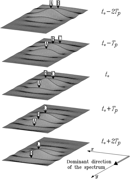
Figure 9.1 shows some pictures of the deterministic wave function (9.2). Point x_o,y_o of the wave of given exceptionally large height H is at the center of the framed area. The input data are: deep water; spectrum: mean JONSWAP; directional distribution: Mitsuyasu et al. with n_p = 20; dominant direction parallel to the y-axis. We see a three-dimensional wave group transiting x_o,y_o. Thus, the theory implicitly reveals the existence of a well-defined physical unit, that is, the three-dimensional wave group. The theory also reveals two basic features of this group. First, the individual waves have a propagation speed greater than the group velocity, so that each of them runs along the envelope from the tail where it is born to the head where it dies (follow wave B during its evolution). Second, the wave group has a development stage that is followed by a decay stage; in the development stage the three-dimensional envelope shrinks, so that the height of the central wave grows to a maximum.

FIGURE 9.1 In the open sea, deterministic wave function (8.83) represents a wave group that strikes home point x_o,y_o, at the apex of its development stage.

As we may see, the answer of the theory is simple and clear. In words it says: “if you record an exceptionally large wave at a point at sea, you can expect that most probably it is the center of a well-defined group at the apex of its development.”

The wave groups are similar to the human families. Let us think of the house of Medici of Florence. Throughout the fourteenth and fifteenth century this family had a development stage up to a maximum at the age of Lorenzo the Magnificent. Then during the two following centuries the family had a progressive decay. In the four centuries from 1300 AD to 1700 AD a lot of individuals of this family were born, grew up, and died. The same is true of the waves: the group is like the family, and the individual waves are like the members of the family. The wave group at the apex of the development stage is like the house of Medici at the age of Lorenzo the Magnificent, and the wave at the center of the group at the apex of its development is like Lorenzo the Magnificent in the years of his full maturity.

The propagation speed of the wave group is nearly equal to the group velocity c_G (cf. Section 1.10) associated with the period T_p, and the propagation speed of each individual wave is nearly equal to the phase speed c associated with T_p. Therefore, on deep water, the propagation speed of each individual wave is nearly twice the propagation speed of the wave group. The fact that each individual wave moves along the envelope leads to a few amazing transformations: the wave that goes to occupy the central position of the group at the apex of the development stage nearly doubles its height in a run of only one wavelength! Moreover, as an individual wave approaches the central position of the group, its wave period and wavelength reduce itself. As it leaves the central position, a compensating stretch occurs.

In Fig. 9.1 we see first the replacement of wave A by wave B at the envelope center, and then the replacement of wave B by wave C. At sea the replacement at the envelope center sometimes becomes well evident. This occurs if a large wave like A in the first image of Fig. 9.1 is spilling near the crest. Then this wave leaves the central position (second image), it gets smaller, and it sheds its whitecap. Then the next wave (B) takes the central position, and it starts spilling near the crest. Then, wave B leaves the central position, which is occupied by the next wave (C), and this wave in its turn starts spilling near the crest. In these cases the whitecap is like a crown passing from one wave to the next one.

9.1.2. The Core of the Quasi-Determinism Theory

We shall call G1 the deterministic wave group given by Eqn (9.1), and G2 the deterministic wave group given by Eqn (9.2). The sequence of pictures of G1 looks essentially like the sequence of pictures of G2.

However, there are some differences. Figure 9.2 shows these two wave groups in the time domain at point x_o,y_o (they represent the records that would be done by an ideal gauge at point x_o,y_o at the center of the framed area). The reason for this difference is the following:

FIGURE 9.2 Wave group G1 and wave group G2 at point x_o,y_o, in the time domain.

A wave group yields its maximum crest elevation at a point 1 and its maximum wave height at a point 2 somewhat after point 1. At point 1 the envelope center coincides with the wave crest. Then the wave crest is reduced because it leaves the envelope center, and the following trough grows because it approaches the envelope center. At point 2 the envelope center coincides with the zero between the crest and the trough. The quasi-determinism (QD) theory says “if you record a wave crest at a fixed point x_o,y_o, with a given exceptionally large height b, you may expect that most probably your point x_o,y_o is point 1”; and “if you record a wave at a fixed point x_o,y_o, with a given exceptionally large height H, you may expect that most probably your point x_o,y_o is point 2.”

Is this the only difference between G2 and G1? It is not exactly so. We have seen that a wave group has a development stage in which the three-dimensional envelope shrinks, and a decay stage in which the three-dimensional envelope stretches. Well, wave group G1 gets the apex of its development stage at the very instant wherein the envelope center transits at point 1 (which gives a further small contribution to yield the exceptional crest elevation at point 1); whereas G2 gets the apex of its development stage at the instant wherein the envelope centre transits at point 2 (which gives a further small contribution to yield the exceptional wave height at point 2).

Thus the full response of the theory is, first: “if you record a wave crest at a fixed point x_o,y_o, with a given exceptionally large height b, you may expect that most probably your point x_o,y_o is point 1, and that the wave group has got the apex of its development at the very instant wherein the envelope center transits at point 1”; second: “if you record a wave at a fixed point x_o,y_o, with a given exceptionally large height H, you may expect that most probably your point x_o,y_o is point 2, and that the wave group has got the apex of its development at the very instant wherein the envelope center transits at point 2.” Now we can appreciate the overall consistency between Eqns (8.17) and (8.41): the first represents wave group G1 in the time domain at point x_o,y_o; the second represents wave group G2 in the time domain at point x_o,y_o.

9.2. Particle Velocity and Acceleration in Wave Groups

The deterministic velocity potential associated to wave groups (8.75) and (8.83) is given, respectively, by Eqns (8.76) and (8.84). With Eqn (7.30) of the cross-covariance,

\bar{ϕ}

$\bar{ϕ}$

becomes, respectively

$\bar{ϕ} (x_{o} + X, y_{o} + Y, z, t_{o} + T) = g b \int_{0}^{\infty} \int_{0}^{2 π} S (ω, θ) ω^{- 1} \frac{\cosh [k (d + z)]}{\cosh (k d)} \sin (k X \sin θ + k Y \cos θ - ω T) d θ d ω / \int_{0}^{\infty} \int_{0}^{2 π} S (ω, θ) d θ d ω$ $\bar{ϕ} (x_{o} + X, y_{o} + Y, z, t_{o} + T) = g b \int_{0}^{\infty} \int_{0}^{2 π} S (ω, θ) ω^{- 1} \frac{\cosh [k (d + z)]}{\cosh (k d)} \sin (k X \sin θ + k Y \cos θ - ω T) d θ d ω / \int_{0}^{\infty} \int_{0}^{2 π} S (ω, θ) d θ d ω$

(9.3)

$\bar{ϕ} (x_{o} + X, y_{o} + Y, z, t_{o} + T) = g \frac{H}{2} \int_{0}^{\infty} \int_{0}^{2 π} S (ω, θ) ω^{- 1} \frac{\cosh [k (d + z)]}{\cosh (k d)} {\sin (k X \sin θ + k Y \cos θ - ω T) - \sin [k X \sin θ + k Y \cos θ - ω (T - T^{*})]} d θ d ω / \int_{0}^{\infty} \int_{0}^{2 π} S (ω, θ) [1 - \cos (ω T^{*})] d θ d ω$ $\bar{ϕ} (x_{o} + X, y_{o} + Y, z, t_{o} + T) = g \frac{H}{2} \int_{0}^{\infty} \int_{0}^{2 π} S (ω, θ) ω^{- 1} \frac{\cosh [k (d + z)]}{\cosh (k d)} {\sin (k X \sin θ + k Y \cos θ - ω T) - \sin [k X \sin θ + k Y \cos θ - ω (T - T^{*})]} d θ d ω / \int_{0}^{\infty} \int_{0}^{2 π} S (ω, θ) [1 - \cos (ω T^{*})] d θ d ω$

(9.4)

Particle velocity and acceleration in the wave groups proceed on differentiating these functions

\bar{ϕ}

$\bar{ϕ}$

. We have:

Wave Group G1

$\bar{v_{x}} (x_{o} + X, y_{o} + Y, z, t_{o} + T) = g b \int_{0}^{\infty} \int_{0}^{2 π} S (ω, θ) k \sin θ ω^{- 1} \frac{\cosh [k (d + z)]}{\cosh (k d)} \cdot \cos (k X \sin θ + k Y \cos θ - ω T) d θ d ω / \int_{0}^{\infty} \int_{0}^{2 π} S (ω, θ) d θ d ω$ $\bar{v_{x}} (x_{o} + X, y_{o} + Y, z, t_{o} + T) = g b \int_{0}^{\infty} \int_{0}^{2 π} S (ω, θ) k \sin θ ω^{- 1} \frac{\cosh [k (d + z)]}{\cosh (k d)} \cdot \cos (k X \sin θ + k Y \cos θ - ω T) d θ d ω / \int_{0}^{\infty} \int_{0}^{2 π} S (ω, θ) d θ d ω$

(9.5)

$\bar{v_{y}} (x_{o} + X, y_{o} + Y, z, t_{o} + T) = g b \int_{0}^{\infty} \int_{0}^{2 π} S (ω, θ) k \cos θ ω^{- 1} \frac{\cosh [k (d + z)]}{\cosh (k d)} \cdot \cos (k X \sin θ + k Y \cos θ - ω T) d θ d ω / \int_{0}^{\infty} \int_{0}^{2 π} S (ω, θ) d θ d ω$ $\bar{v_{y}} (x_{o} + X, y_{o} + Y, z, t_{o} + T) = g b \int_{0}^{\infty} \int_{0}^{2 π} S (ω, θ) k \cos θ ω^{- 1} \frac{\cosh [k (d + z)]}{\cosh (k d)} \cdot \cos (k X \sin θ + k Y \cos θ - ω T) d θ d ω / \int_{0}^{\infty} \int_{0}^{2 π} S (ω, θ) d θ d ω$

(9.6)

$\bar{v_{z}} (x_{o} + X, y_{o} + Y, z, t_{o} + T) = g b \int_{0}^{\infty} \int_{0}^{2 π} S (ω, θ) k ω^{- 1} \frac{\sinh [k (d + z)]}{\cosh (k d)} \cdot \sin (k X \sin θ + k Y \cos θ - ω T) d θ d ω / \int_{0}^{\infty} \int_{0}^{2 π} S (ω, θ) d θ d ω$ $\bar{v_{z}} (x_{o} + X, y_{o} + Y, z, t_{o} + T) = g b \int_{0}^{\infty} \int_{0}^{2 π} S (ω, θ) k ω^{- 1} \frac{\sinh [k (d + z)]}{\cosh (k d)} \cdot \sin (k X \sin θ + k Y \cos θ - ω T) d θ d ω / \int_{0}^{\infty} \int_{0}^{2 π} S (ω, θ) d θ d ω$

(9.7)

$\bar{a_{x}} (x_{o} + X, y_{o} + Y, z, t_{o} + T) = g b \int_{0}^{\infty} \int_{0}^{2 π} S (ω, θ) k \sin θ \frac{\cosh [k (d + z)]}{\cosh (k d)} \cdot \sin (k X \sin θ + k Y \cos θ - ω T) d θ d ω / \int_{0}^{\infty} \int_{0}^{2 π} S (ω, θ) d θ d ω$ $\bar{a_{x}} (x_{o} + X, y_{o} + Y, z, t_{o} + T) = g b \int_{0}^{\infty} \int_{0}^{2 π} S (ω, θ) k \sin θ \frac{\cosh [k (d + z)]}{\cosh (k d)} \cdot \sin (k X \sin θ + k Y \cos θ - ω T) d θ d ω / \int_{0}^{\infty} \int_{0}^{2 π} S (ω, θ) d θ d ω$

(9.8)

$\bar{a_{y}} (x_{o} + X, y_{o} + Y, z, t_{o} + T) = g b \int_{0}^{\infty} \int_{0}^{2 π} S (ω, θ) k \cos θ \frac{\cosh [k (d + z)]}{\cosh (k d)} \cdot \sin (k X \sin θ + k Y \cos θ - ω T) d θ d ω / \int_{0}^{\infty} \int_{0}^{2 π} S (ω, θ) d θ d ω$ $\bar{a_{y}} (x_{o} + X, y_{o} + Y, z, t_{o} + T) = g b \int_{0}^{\infty} \int_{0}^{2 π} S (ω, θ) k \cos θ \frac{\cosh [k (d + z)]}{\cosh (k d)} \cdot \sin (k X \sin θ + k Y \cos θ - ω T) d θ d ω / \int_{0}^{\infty} \int_{0}^{2 π} S (ω, θ) d θ d ω$

(9.9)

$\bar{a_{z}} (x_{o} + X, y_{o} + Y, z, t_{o} + T) = - g b \int_{0}^{\infty} \int_{0}^{2 π} S (ω, θ) k \frac{\sinh [k (d + z)]}{\cosh (k d)} \cdot \cos (k X \sin θ + k Y \cos θ - ω T) d θ d ω / \int_{0}^{\infty} \int_{0}^{2 π} S (ω, θ) d θ d ω$ $\bar{a_{z}} (x_{o} + X, y_{o} + Y, z, t_{o} + T) = - g b \int_{0}^{\infty} \int_{0}^{2 π} S (ω, θ) k \frac{\sinh [k (d + z)]}{\cosh (k d)} \cdot \cos (k X \sin θ + k Y \cos θ - ω T) d θ d ω / \int_{0}^{\infty} \int_{0}^{2 π} S (ω, θ) d θ d ω$

(9.10)

Wave Group G2

$\bar{v_{x}} (x_{o} + X, y_{o} + Y, z, t_{o} + T) = g \frac{H}{2} \int_{0}^{\infty} \int_{0}^{2 π} S (ω, θ) k \sin θ ω^{- 1} \frac{\cosh [k (d + z)]}{\cosh (k d)} \cdot {\cos (k X \sin θ + k Y \cos θ - ω T) - \cos [k X \sin θ + k Y \cos θ - ω (T - T^{*})]} d θ d ω / \int_{0}^{\infty} \int_{0}^{2 π} S (ω, θ) [1 - \cos (ω T^{*})] d θ d ω$ $\bar{v_{x}} (x_{o} + X, y_{o} + Y, z, t_{o} + T) = g \frac{H}{2} \int_{0}^{\infty} \int_{0}^{2 π} S (ω, θ) k \sin θ ω^{- 1} \frac{\cosh [k (d + z)]}{\cosh (k d)} \cdot {\cos (k X \sin θ + k Y \cos θ - ω T) - \cos [k X \sin θ + k Y \cos θ - ω (T - T^{*})]} d θ d ω / \int_{0}^{\infty} \int_{0}^{2 π} S (ω, θ) [1 - \cos (ω T^{*})] d θ d ω$

(9.11)

$\bar{v_{y}} (x_{o} + X, y_{o} + Y, z, t_{o} + T) = g \frac{H}{2} \int_{0}^{\infty} \int_{0}^{2 π} S (ω, θ) k \cos θ ω^{- 1} \frac{\cosh [k (d + z)]}{\cosh (k d)} \cdot {\cos (k X \sin θ + k Y \cos θ - ω T) - \cos [k X \sin θ + k Y \cos θ - ω (T - T^{*})]} d θ d ω / \int_{0}^{\infty} \int_{0}^{2 π} S (ω, θ) [1 - \cos (ω T^{*})] d θ d ω$ $\bar{v_{y}} (x_{o} + X, y_{o} + Y, z, t_{o} + T) = g \frac{H}{2} \int_{0}^{\infty} \int_{0}^{2 π} S (ω, θ) k \cos θ ω^{- 1} \frac{\cosh [k (d + z)]}{\cosh (k d)} \cdot {\cos (k X \sin θ + k Y \cos θ - ω T) - \cos [k X \sin θ + k Y \cos θ - ω (T - T^{*})]} d θ d ω / \int_{0}^{\infty} \int_{0}^{2 π} S (ω, θ) [1 - \cos (ω T^{*})] d θ d ω$

(9.12)

$\bar{v_{z}} (x_{o} + X, y_{o} + Y, z, t_{o} + T) = g \frac{H}{2} \int_{0}^{\infty} \int_{0}^{2 π} S (ω, θ) k ω^{- 1} \frac{\sinh [k (d + z)]}{\cosh (k d)} \cdot {\sin (k X \sin θ + k Y \cos θ - ω T) - \sin [k X \sin θ + k Y \cos θ - ω (T - T^{*})]} d θ d ω / \int_{0}^{\infty} \int_{0}^{2 π} S (ω, θ) [1 - \cos (ω T^{*})] d θ d ω$ $\bar{v_{z}} (x_{o} + X, y_{o} + Y, z, t_{o} + T) = g \frac{H}{2} \int_{0}^{\infty} \int_{0}^{2 π} S (ω, θ) k ω^{- 1} \frac{\sinh [k (d + z)]}{\cosh (k d)} \cdot {\sin (k X \sin θ + k Y \cos θ - ω T) - \sin [k X \sin θ + k Y \cos θ - ω (T - T^{*})]} d θ d ω / \int_{0}^{\infty} \int_{0}^{2 π} S (ω, θ) [1 - \cos (ω T^{*})] d θ d ω$

(9.13)

$\bar{a_{x}} (x_{o} + X, y_{o} + Y, z, t_{o} + T) = g \frac{H}{2} \int_{0}^{\infty} \int_{0}^{2 π} S (ω, θ) k \sin θ \frac{\cosh [k (d + z)]}{\cosh (k d)} \cdot {\sin (k X \sin θ + k Y \cos θ - ω T) - \sin [k X \sin θ + k Y \cos θ - ω (T - T^{*})]} d θ d ω / \int_{0}^{\infty} \int_{0}^{2 π} S (ω, θ) [1 - \cos (ω T^{*})] d θ d ω$ $\bar{a_{x}} (x_{o} + X, y_{o} + Y, z, t_{o} + T) = g \frac{H}{2} \int_{0}^{\infty} \int_{0}^{2 π} S (ω, θ) k \sin θ \frac{\cosh [k (d + z)]}{\cosh (k d)} \cdot {\sin (k X \sin θ + k Y \cos θ - ω T) - \sin [k X \sin θ + k Y \cos θ - ω (T - T^{*})]} d θ d ω / \int_{0}^{\infty} \int_{0}^{2 π} S (ω, θ) [1 - \cos (ω T^{*})] d θ d ω$

(9.14)

$\bar{a_{y}} (x_{o} + X, y_{o} + Y, z, t_{o} + T) = g \frac{H}{2} \int_{0}^{\infty} \int_{0}^{2 π} S (ω, θ) k \cos θ \frac{\cosh [k (d + z)]}{\cosh (k d)} \cdot {\sin (k X \sin θ + k Y \cos θ - ω T) - \sin [k X \sin θ + k Y \cos θ - ω (T - T^{*})]} d θ d ω / \int_{0}^{\infty} \int_{0}^{2 π} S (ω, θ) [1 - \cos (ω T^{*})] d θ d ω$ $\bar{a_{y}} (x_{o} + X, y_{o} + Y, z, t_{o} + T) = g \frac{H}{2} \int_{0}^{\infty} \int_{0}^{2 π} S (ω, θ) k \cos θ \frac{\cosh [k (d + z)]}{\cosh (k d)} \cdot {\sin (k X \sin θ + k Y \cos θ - ω T) - \sin [k X \sin θ + k Y \cos θ - ω (T - T^{*})]} d θ d ω / \int_{0}^{\infty} \int_{0}^{2 π} S (ω, θ) [1 - \cos (ω T^{*})] d θ d ω$

(9.15)

$\bar{a_{z}} (x_{o} + X, y_{o} + Y, z, t_{o} + T) = - g \frac{H}{2} \int_{0}^{\infty} \int_{0}^{2 π} S (ω, θ) k \frac{\sinh [k (d + z)]}{\cosh (k d)} \cdot {\cos (k X \sin θ + k Y \cos θ - ω T) - \cos [k X \sin θ + k Y \cos θ - ω (T - T^{*})]} d θ d ω / \int_{0}^{\infty} \int_{0}^{2 π} S (ω, θ) [1 - \cos (ω T^{*})] d θ d ω$ $\bar{a_{z}} (x_{o} + X, y_{o} + Y, z, t_{o} + T) = - g \frac{H}{2} \int_{0}^{\infty} \int_{0}^{2 π} S (ω, θ) k \frac{\sinh [k (d + z)]}{\cosh (k d)} \cdot {\cos (k X \sin θ + k Y \cos θ - ω T) - \cos [k X \sin θ + k Y \cos θ - ω (T - T^{*})]} d θ d ω / \int_{0}^{\infty} \int_{0}^{2 π} S (ω, θ) [1 - \cos (ω T^{*})] d θ d ω$

(9.16)

If the wave of the given height H very large is a zero down-crossing wave, both Eqn (9.2) of

\bar{η}

$\bar{η}$

and Eqns (9.11)–(9.16) of

\bar{v_{x}}

$\bar{v_{x}}$

\bar{v_{y}}

$\bar{v_{y}}$

\bar{v_{z}}

$\bar{v_{z}}$

\bar{a_{x}}

$\bar{a_{x}}$

\bar{a_{y}}

$\bar{a_{y}}$

\bar{a_{z}}

$\bar{a_{z}}$

must be multiplied by (−1).

The knowledge of particle velocities and accelerations enables us to calculate the wave loads on cylinders of small diameter, by means of the Morison equation (as we shall see in Chapter 12). Then the knowledge of particle accelerations enables us to calculate the Froude-Krylov forces on isolated bodies. As we have already seen in Chapter 2, the Froude-Krylov force is the force acting on an ideal water body with the same volume and shape as the solid body. As such, the Froude-Krylov force is related to a_x, a_y, a_z by

$F = \int_{W} ρ (a_{x} i_{x} + a_{y} i_{y} + a_{z} i_{z}) d W$ $F = \int_{W} ρ (a_{x} i_{x} + a_{y} i_{y} + a_{z} i_{z}) d W$

(9.17)

where W denotes the volume of the water body. Calculation of the Froude-Krylov force is a preliminary step that is necessary for calculating wave loads on large isolated bodies with an arbitrary shape. In Chapter 10 we shall see which calculation must be done for passing from the Froude-Krylov force to the actual wave force on the solid body. Then, in Chapter 13 we shall see some examples of calculations of wave loads on large isolated bodies.

Typically, we shall assume

$H = H_{\max} or b = b_{\max}$ $H = H_{\max} or b = b_{\max}$

(9.18)

where H_max and b_max are, respectively, the maximum expected wave height and the maximum expected crest elevation in the design sea state (Chapter 5). With Eqns (9.11)–(9.16) we shall be able to calculate the effect of the wave with the maximum expected height, and with Eqns (9.5)–(9.10) we shall be able to calculate the effect of the wave crest with the maximum expected height.

9.3. The Subroutine QD

The inputs are X, Y, z, T, and UD (if the wave of the given very large height H is a zero up-crossing → UD = 1; otherwise, UD = −1). NCALL must be 1, except for a preliminary call, as we shall see later.

The outputs are

\bar{η}

$\bar{η}$

\bar{v_{x}}

$\bar{v_{x}}$

\bar{v_{y}}

$\bar{v_{y}}$

\bar{v_{z}}

$\bar{v_{z}}$

\bar{a_{x}}

$\bar{a_{x}}$

\bar{a_{y}}

$\bar{a_{y}}$

\bar{a_{z}}

$\bar{a_{z}}$

. The subroutine is specified for the mean JONSWAP spectrum, and the directional distribution of Mitsuyasu et al. However, for changing the spectrum or the directional distribution one has to operate on a small number of variables, which are those included between the two lines of asterisks.

The program must supply: d, H_s, H, A, θ_d, and n_p. (Alternatively, the program may give T_p in place of H_s and A. In this case one has to cancel a pair of lines from the subroutine, which serve to obtain T_p from H_s and A.)

A preliminary call of the subroutine must be done with NCALL = 0. This serves to compute the directional spectrum S(ω, θ) with steps dω, dθ suitable for the numerical integrations. The values of S(ω, θ) are stored on memory (SOT(I,J)) for the next calls of the subroutine.

The calculation is made with Eqns (9.2) and (9.11)–(9.16). All of the output variables are the result of the ratio of two integrals with respect to ω and θ. The integral in the denominator is the same for the whole set of variables and is denoted by DENOINT. The integral in the numerator is denoted ETAINT, VXINT, VYINT, etc.

Program EXAMPLE shows an easy application, with the inputs of subroutine QD being given from the console.

  SUBROUTINE QD(NCALL,UD,X,Y,Z,T,VX,VY,VZ,AX,AY,AZ,ETA)
  COMMON D,HS,H,TP,TST,ALPHA, TETAD,RNP
  COMMON IMAX,JMAX,OMV(300),TETV(150),RKV(300)
  COMMON SOT(300,150)
  DIMENSION EO(300),DTE(150)
  G=9.8
  G2=G∗G
  PG=3.141592
  DPG=2.∗PG
  IF(NCALL.GT.0)GO TO 500
c∗∗∗∗∗∗∗∗∗∗∗∗∗∗∗∗∗∗∗∗∗∗∗∗∗∗∗∗∗∗∗∗∗∗∗∗∗∗∗∗∗∗∗
  RK0=1.345
  CHI1=3.3
  CHI2=0.08
  CST=0.44
c∗∗∗∗∗∗∗∗∗∗∗∗∗∗∗∗∗∗∗∗∗∗∗∗∗∗∗∗∗∗∗∗∗∗∗∗∗∗∗∗∗∗∗

  COST=RK0/ALPHA∗∗0.25
  TP=COST∗PG∗SQRT(HS/G)
  TST=CST∗TP
  ALCHI1=ALOG(CHI1)
  CHI2Q=CHI2∗CHI2
  OMP=DPG/TP
  DOMEGA=OMP/50.
  O1=0.5∗OMP
  O2=3.∗OMP
  OMPQ=OMP∗OMP
  DTETA=PG/100.
  TE1=-PG/2.
  TE2=PG/2.
  OM=O1-DOMEGA/2.
  I=0
c Loop 90: the grid of values of the directional spectrum, being necessary
c for the execution of the double integrals, is loaded on memory
90   OM=OM+DOMEGA
  IF(OM.GT.O2)GO TO 91
  I=I+1
  OMV(I)=OM
c values of omega stored on OMV(I) (I=1,IMAX)
  PE=DPG/OM
  RL0=(G/DPG)∗PE∗PE
  DL0=D/RL0
  IF(DL0.GT.0.5)THEN
  RKV(I)=DPG/RL0
  ELSE
  RLP=RL0
300   RL=RL0∗TANH(DPG∗D/RLP)
  TES=ABS(RL-RLP)/RL
  RLP=RL
  IF(TES.GT.1.E-4)GO TO 300
  RKV(I)=DPG/RL
  ENDIF
c k(omega) stored on RKV(I)
  OMM5=1./OM∗∗5
  ARG=(OM-OMP)∗∗2/(2.∗CHI2Q∗OMPQ)
  E3=EXP(-ARG)
  ARG=ALCHI1∗E3
  E2=EXP(ARG)
  ARG=1.25∗(OMP/OM)∗∗4
  E1=EXP(-ARG)
  EO(I)=ALPHA∗G2∗OMM5∗E1∗E2
c EO(I)=SSE(omega)
c∗∗∗∗∗∗∗∗∗∗∗∗∗∗∗∗∗∗∗∗∗∗∗∗∗∗∗∗∗∗∗∗∗∗∗∗∗∗∗∗∗∗∗

  IF(OM.LE.OMP)THEN
  RN=RNP∗(OM/OMP)∗∗5
  ELSE
  RN=RNP∗(OMP/OM)∗∗2.5
  ENDIF
c∗∗∗∗∗∗∗∗∗∗∗∗∗∗∗∗∗∗∗∗∗∗∗∗∗∗∗∗∗∗∗∗∗∗∗∗∗∗∗∗∗∗∗∗∗
  DN=2.∗RN
  TE=TE1-DTETA/2
  J=0
80    TE=TE+DTETA
  IF(TE.GT.TE2)GO TO 81
  J=J+1
  TETV(J)=TE+TETAD
c values of theta stored on TETV(J) (J=1,JMAX)
  ABC=ABS(COS(TE/2.))
  DTE(J)=ABC∗∗DN
  GO TO 80
81   CONTINUE
  JMAX=J
  SOMT=0
  DO J=1,JMAX
  SOMT=SOMT+DTE(J)∗DTETA
  ENDDO
  RKN=1./SOMT

c RKN=K(n) (Eqn 6.18)

  DO J=1,JMAX
  DTE(J)=RKN∗DTE(J)
c DTE(J)=D(theta;omega)
  SOT(I,J)=DTE(J)∗EO(I)
c directional spectrum stored on SOT(I,J)
  ENDDO
  GO TO 90
91   CONTINUE
  IMAX=I
  IF(NCALL.EQ.0)GO TO 501
500   CONTINUE

c ETAINT=double integral numerator RHS of Eqn (9.2)

c VXINT=double integral numerator RHS of Eqn (9.5)

c VYINT=double integral numerator RHS of Eqn (9.6)

c VZINT=double integral numerator RHS of Eqn (9.7)

c AXINT=double integral numerator RHS of Eqn (9.8)

c AYINT=double integral numerator RHS of Eqn (9.9)

c AZINT=double integral numerator RHS of Eqn (9.10)

c DENOINT=double integral denominator RHS of Eqn (9.2) or (9.5)–(9.10)

  ETAINT=0
  VXINT=0
  VYINT=0

  .VZINT=0
  AXINT=0
  AYINT=0
  AZINT=0
  DENOINT=0
  DO I=1,IMAX
  DO J=1,JMAX
  OM=OMV(I)
  OM1=1./OM
  RK=RKV(I)
c A1 attenuation factor of horizontal components
c A2 attenuation factor of vertical components
c for large kd both A1 and A2 tend to exp(kz). This
c asymptotic form is used (for large kd) in order to avoid
c overflow errors in cosh(kd)
  IF(RK∗D.GT.20)THEN
  A1=EXP(RK∗Z)
  A2=A1
  ELSE
  A1=COSH(RK∗(D+Z))/COSH(RK∗D)
  A2=SINH(RK∗(D+Z))/COSH(RK∗D)
  ENDIF
  TE=TETV(J)
  S=SOT(I,J)
  ST=SIN(TE)
  CT=COS(TE)
  ARG1=RK∗X∗ST+RK∗Y∗CT-OM∗T
  ARG2=RK∗X∗ST+RK∗Y∗CT-OM∗(T-TST)
  CO1=COS(ARG1)
  CO2=COS(ARG2)
  SI1=SIN(ARG1)
  SI2=SIN(ARG2)
  ETAINT=ETAINT+S∗(CO1-CO2)
  VXINT=VXINT+S∗OM1∗RK∗A1∗ST∗(CO1-CO2)
  VYINT=VYINT+S∗OM1∗RK∗A1∗CT∗(CO1-CO2)
  VZINT=VZINT+S∗OM1∗RK∗A2∗(SI1-SI2)
  AXINT=AXINT+S∗RK∗A1∗ST∗(SI1-SI2)
  AYINT=AYINT+S∗RK∗A1∗CT∗(SI1-SI2)
  AZINT=AZINT-S∗RK∗A2∗(CO1-CO2)
  DENOINT=DENOINT+S∗(1.-COS(OM∗TST))
  ENDDO
  ENDDO
  ETA=UD∗0.5∗H∗ETAINT/DENOINT
  VX=UD∗0.5∗G∗H∗VXINT/DENOINT
  VY=UD∗0.5∗G∗H∗VYINT/DENOINT
  VZ=UD∗0.5∗G∗H∗VZINT/DENOINT
  AX=UD∗0.5∗G∗H∗AXINT/DENOINT

  .AY=UD∗0.5∗G∗H∗AYINT/DENOINT
  AZ=UD∗0.5∗G∗H∗AZINT/DENOINT
501   CONTINUE
c the values of all the double integrals (ETAINT, VXINT,VYINT, VZINT,
c AXINT, AYINT,AZINT,DENOINT) should have been multiplied by the
c product DTETA∗DOMEGA; however this product cancels on executing
c the ratios ETAINT/DENOINT, VXINT/DENOINT, etc
  RETURN
  END
  PROGRAM EXAMPLE
  COMMON D,HS,H,TP,TST,ALPHA,TETAD,RNP
  COMMON IMAX,JMAX,OMV(300),TETV(150),RKV(300)
  COMMON SOT(300,150)
  PG=3.141592
  DPG=2.∗PG
  WRITE(6,∗)'d,Hs,H'
  READ(5,∗)D,HS,H
  WRITE(6,∗)'alpha,thetad(degree),np'
  READ(5,∗)ALPHA,TETAD,RNP
  WRITE(6,∗)'zero up-crossing wave -> 1, down-crossing -> -1'
  READ(5,∗)UD
  TETAD=TETAD∗PG/180.
  CALL QD(NCALL,UD,X,Y,Z,T,VX,VY,VZ,AX,AY,AZ,ETA)
  NCALL=NCALL+1
500   WRITE(6,∗)'X,Y,Z,T'
  READ(5,∗)X,Y,Z,T
  CALL QD(NCALL,UD,X,Y,Z,T,VX,VY,VZ,AX,AY,AZ,ETA)
  WRITE(6,1000)ETA
  WRITE(6,1001)VX,VY,VZ
  WRITE(6,1001)AX,AY,AZ
1000 FORMAT(2X,F7.2)
1001 FORMAT(2X,3(F7.2,1X))
  GO TO 500
  END

9.4. Experimental Verification of the Quasi-Determinism Theory: Basic Concepts

9.4.1. Obtaining the Deterministic Wave Function from Time Series Data

Let us imagine two wave gauges at two points A and B in a sea area. We measure the surface elevation at these two points in the same time instants. The sample interval is Δt, and n is the number of samples per record per gauge. We wonder “what may we expect to happen at point B provided that a wave with a given height H, being exceptionally large with respect to the sea state, occurs at point A?” According to the QD theory, point A is x_o,y_o and point B is x_o + X,y_o + Y. The expected surface elevation at x_o + X,y_o + Y is given by Eqn (8.83). Using the definition (7.1) of Ψ, Eqn (8.83) may be rewritten in the form

$\bar{η_{B}} (t_{o} + T) = \frac{< η_{A} (t) η_{B} (t + T) > - < η_{A} (t) η_{B} (t + T - T^{*}) >}{< η_{A}^{2} (t) > - < η_{A} (t) η_{A} (t + T^{*}) >} \frac{H}{2}$ $\bar{η_{B}} (t_{o} + T) = \frac{< η_{A} (t) η_{B} (t + T) > - < η_{A} (t) η_{B} (t + T - T^{*}) >}{< η_{A}^{2} (t) > - < η_{A} (t) η_{A} (t + T^{*}) >} \frac{H}{2}$

(9.19)

where

$η_{A} (t) = η (x_{o}, y_{o}, t)$ $η_{A} (t) = η (x_{o}, y_{o}, t)$

(9.20)

$η_{B} (t) = η (x_{o} + X, y_{o} + Y, t)$ $η_{B} (t) = η (x_{o} + X, y_{o} + Y, t)$

(9.21)

and T^∗ is the lag of the absolute minimum of the autocovariance

$ψ (T) = < η_{A} (t) η_{A} (t + T) >$ $ψ (T) = < η_{A} (t) η_{A} (t + T) >$

(9.22)

The averages in Eqn (9.19) may be obtained from the time series data. As an example, let Δt = 0.1 s and n = 3001 as it is currently taken at the NOEL; then for obtaining

{\bar{η}}_{B} (t_{o} + T)

${\bar{η}}_{B} (t_{o} + T)$

with T = 0.6 s we shall have to perform the following average:

$< η_{A} (t) η_{B} (t + 0.6 s) > = \frac{η_{A_{1}} η_{B_{7}} + η_{A_{2}} η_{B_{8}} + \dots + η_{A_{2995}} η_{B_{3001}}}{2995}$ $< η_{A} (t) η_{B} (t + 0.6 s) > = \frac{η_{A_{1}} η_{B_{7}} + η_{A_{2}} η_{B_{8}} + \dots + η_{A_{2995}} η_{B_{3001}}}{2995}$

(9.23)

where

η_{A_{i}}

$η_{A_{i}}$

denotes the ith sample value at point A.

9.4.2. Resorting to Time Series Data of Pressure Head Waves

Equation (9.19) holds also for pressure head waves at some depth beneath the water level. More generally, all that has been shown until now holds whether η is the surface elevation or the fluctuating pressure head at some fixed depth beneath the water level. Hence, one may test the theory either with surface waves or with pressure head waves, at one's own choice. Working with pressure head waves is preferable. Aside from the fact that the author attracted to pressure head waves, there is the fact that, at the NOEL, the cost of a small-scale field experiment (SSFE) on pressure head waves is an order of magnitude smaller than the cost of the same SSFE on surface waves.

9.4.3. A Typical Experiment Aimed to Verify the Theory

There is an array of gauges. The largest distance between two gauges is within a few wave lengths. These gauges record the surface elevation at the same time instants. Many records are taken in many sea states. The largest ratio H/σ is searched in each record. This is the largest value of H/σ from all the zero up-crossing waves and all the zero down-crossing waves obtained by the whole array of gauges in the record. This will be called (H/σ)_{max i}, where i denotes the number of the record. To fix the ideas let us think of these numbers:

number of gauges: 30

record duration: 300 s

number of records: 1000

Let us imagine that the largest value of the ratio (H/σ)_{max i} has occurred in the record i = 600 at t_o = 200 s, that the record was done by gauge number 25, and that the wave of this largest H/σ was a zero up-crossing wave. Then we apply Eqn (9.19) with A = point of gauge 25, and B = point of gauge 1, then B = point of gauge 2, and so on, until B = point of gauge 30. Of course, the time series data used for the averages in Eqn (9.19) will be those of record number 600. Thus, we obtain the

\bar{η} (t_{o} + T)

$\bar{η} (t_{o} + T)$

at the 30 points of the wave gauges, as a function of the time lag T (T typically ranges from −3T_p to 3T_p). Finally, the deterministic

\bar{η}

$\bar{η}$

is compared to the random η in record number 600.

9.5. Results of Small-Scale Field Experiments

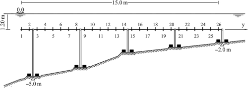
In an early SSFE in 1990 there were nine piles, each of which supported a wave gauge (the plan of the piles is shown in Fig. 9.3). The wave with the largest ratio H/σ was recorded at point 3. It was a zero down-crossing wave with a H/σ = 9.6.

Figure 9.4(a) shows the deterministic

\bar{η} (t_{o} + T)

$\bar{η} (t_{o} + T)$

calculated with Eqn (9.19), and Fig. 9.4(b) shows the random η(t) at the locations of the gauges. The relative phases at the traverse of points 1–7 reveal that the angle between the direction of wave advance (of the deterministic wave) and the y-axis was about 10°. Hence, if the center of the wave crest passed at point 3 it had to pass very close to point 9. At point 9, A is at the center of the envelope, and B is in the envelope tail. At point 3, B is at the center of the envelope, and A is in the envelope head.

FIGURE 9.3 Plan of the wave gauges in the SSFE of 1990 aimed to verify the QD theory.
(The data acquisition system had eight channels so that one of the wave gauges had to be disconnected. In the stage of the experiment wherein the largest wave height occurred, the disconnected gauge was no. 6.)

FIGURE 9.4 SSFE of 1990
(see the plan of the gauges in Fig. 9.3). The figure compares the actual waves (b) with deterministic waves (a) when the wave with the largest H/σ was recorded (this was a zero down-crossing wave with H/σ = 9.6 recorded by gauge no. 3).

Of course, there are some differences between random η and deterministic

\bar{η}

$\bar{η}$

and indeed the QD theory states that η becomes asymptotically equal to

\bar{η}

$\bar{η}$

only as H/σ tends to infinity. Besides these main discrepancies due to residual randomness, there are some discrepancies due to nonlinearity effects, which produce some local distortion of the wave profile that cannot be foreseen by the linear QD theory. However, the overall closeness between the random waves (η) and the deterministic waves (

\bar{η}

$\bar{η}$

) was evident since that early experiment of 1990.

The more recent SSFEs deal with waves in the space-time domain. Besides time series at some fixed points, these experiments enable one to obtain wave profiles in the space domain. This is possible because the wave gauges are close to each other and sensibly aligned with the wave direction, as is shown in Fig. 9.5.

This novelty has made it possible to take a step forward into verification of the QD theory. Indeed, some cases were found wherein the overall closeness between random wave profiles and deterministic wave profiles is really amazing. In particular, look at Fig. 9.6, where the continuous lines represent the deterministic wave profiles and the dashed lines represent the random wave profiles, for a case of a ratio H/σ = 9.22. Figure 9.6 proves that the wave groups of the QD theory do exist in the field. The figure shows the transit of one of these groups over the gauge array (GA). In the first line of the figure (t_o − 5 s), on the right-hand side of the GA there is the near-calm that precedes the arrival of a wave group; on the left-hand side there is wave crest A, which is decreasing because it precedes the envelope center. On the opposite in the last line (t_o + 6 s), on the left-hand side of the GA there is the near-calm that follows the transit of a wave group; on the right-hand side there is wave crest E that is growing because it follows the envelope center, which has already left the GA. The envelope center is close to the locations of wave crests B, C, and D, respectively, at t_o − 2 s, t_o + 1 s, and t_o + 4 s. Wave crests B and C nearly complete their life cycle during the passage over the GA. In particular, wave crest B is in its growing stage from t_o − 4 s to t_o − 2 s and in the decay stage from t_o − 2 s to t_o; wave crest C is in its growing stage from t_o − 2 s to t_o + 1 s, and in the decay stage from t_o + 1 s to t_o + 2 s.

FIGURE 9.5 The gauges of a recent SSFE (2010) aimed to verify the QD theory.
There was an array of 26 pressure transducers, each of which was connected with a small vertical tube with a bending section (like a small periscope). Pressure head waves were measured 0.80 m beneath the mean water level.

FIGURE 9.6 Small-scale field experiment of 2010.
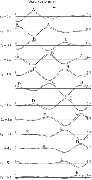
What happened when a zero down-crossing wave of H/σ = 9.22 was recorded by gauge no. 18 (the location of this gauge is shown by a small vertical segment in the picture relevant to time instant t_o). Dashed line: actual (random) wave. Continuous line: deterministic wave.

9.6. Conclusion

The characteristic mechanics of wave groups shown in Section 9.1.1 were disclosed in a paper by the author (1989). Only some years later than the publication of the paper (1989) the author realized the overall physical consistency of the theory, which here has been called “core of the theory” (Section 9.1.2), and was disclosed in the book (2000). The SSFEs of 1990 and 2010 were described, respectively, by Boccotti et al. (1993) and Boccotti (2011).

Two full-scale field experiments on the configuration of wave group G1 near the exceptionally large wave crest were performed by Phillips et al. (1993a,b). Some nonlinearity effects on the wave groups were dealt with by Arena (2005), Arena and Fedele (2005), Fedele and Arena (2005), Arena et al. (2008), and Arena and Guedes Soares (2009). The QD theory has widened the view on sea wave groups: from statistics to mechanics. A wave group was dealt with in the time domain and defined as a sequence of waves with heights greater than some given (large) threshold. The analysis was purely in statistics: concerning the number of waves (Kimura, 1980; van Vledder, 1992; Medina and Huspeth, 1990), or the wave energy of the group (Medina and Hudspeth, 1994).

..................Content has been hidden....................

You can't read the all page of ebook, please click here login for view all page.

Table of Contents for Chapter 9. Quasi-Determinism Theory: Mechanics of Wave Groups

Create new playlist

Sign In

Sign Up

Abstract

Keywords

9.1. What Does the Deterministic Wave Function Represent?

9.1.1. A Three-Dimensional Wave Group

9.1.2. The Core of the Quasi-Determinism Theory

9.2. Particle Velocity and Acceleration in Wave Groups

9.3. The Subroutine QD

9.4. Experimental Verification of the Quasi-Determinism Theory: Basic Concepts

9.4.1. Obtaining the Deterministic Wave Function from Time Series Data

9.4.2. Resorting to Time Series Data of Pressure Head Waves

9.4.3. A Typical Experiment Aimed to Verify the Theory

9.5. Results of Small-Scale Field Experiments

9.6. Conclusion

Table of Contents for
Chapter 9. Quasi-Determinism Theory: Mechanics of Wave Groups