Search in book...
Toggle Font Controls
Create new playlist

Name your new playlist

Playlist description (optional)
Sign In

Email address

Password

Forgot Password?

or

Continue with Facebook

Continue with Google
Sign Up

Full Name

Email address

Confirm Email Address

Password

or

Continue with Facebook

Continue with Google

Chapter 15

Conversion of Wave Energy

Abstract

The chapter starts from a review of wave energy converters from the 1960s to the present day. It points out that the recent U-oscillating water column (OWC) is better than the well-known OWC because of a greater eigenperiod, and because of the possibility of exploiting the experience with caisson breakwaters. However, passing from an OWC to a U-OWC calls for a radical change of calculation, which is dealt with in the chapter. Indeed it is no longer possible to exploit the Stoker solution (1957) for the waves generated by an oscillating pressure applied uniformly over a segment of the water surface. A crucial item of the new solution for the U-OWCs concerns the propagation speed c_R of the reflected wave energy. The chapter shows that, with some swell, c_R may be smaller than the group velocity with the consequence of both super-wave-amplification and superabsorption. Some evidence of this phenomenon is provided from a small-scale field experiment.

Keywords

Absorption coefficient; Fixed OWC; Point absorbers; Small-scale field experiment (SSFE); U-OWC; Wave energy conversion; Wave-converter interaction

15.1. An Overview of Work Done to Exploit Wave Energy Source

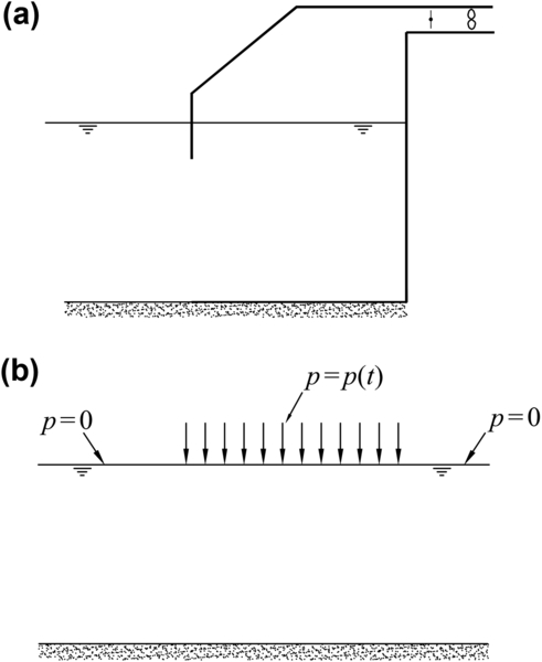
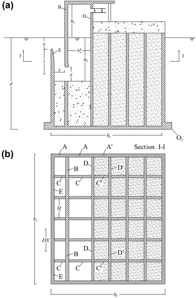
Many immersed oscillating systems have been disclosed for the aim of wave energy conversion. One of the first was a navigation buoy due to the pioneering research of Commander Yoshio Masuda in Japan. It consisted of a battery-charging generator driven by an oscillating water column (OWC) contained in a vertical pipe through a floating buoy. Masuda's developmental work of this device was in the mid-1960s (see ECOR, 2003; Falcao, 2010, for more details). The research of the 1970s concentrated mainly on resonant point absorbers (McCormick, 1974; Mei, 1976; Budal and Falnes, 1975, 1977). Two well-known devices of those years were the “Salter duck” (Salter, 1974) and the “Bristol cylinder” (Evans, 1976). According to the classification of Hagerman (1995), these belong, respectively, to the class of “pitching floats with mutual force reaction” and “submerged buoyant absorbers with sea-floor reaction point.” Starting from the 1980s, most international attention was focused on fixed OWCs, whose prototypes were built in Australia, China, India, Japan, Norway, Portugal, and the United Kingdom. A conventional fixed OWC is essentially a box with a large opening on the wave-beaten wall. This opening usually goes from the seabed to nearly the mean water level (see the scheme of Fig. 15.1(a)). An air pocket remains between the roof and sea surface and is connected to the atmosphere by an exhaust tube with a turbine. Typically, this is a Wells turbine that rotates in the same direction even if the direction of the air flow is reversed (Raghunathan, 1995). Calculation of the performances of these kind of plants (Evans, 1982; Sarmento and Falcao, 1985) is founded on one pillar, that is, Stoker's solution (1957) for the waves generated by an oscillating pressure applied uniformly over a segment of the water surface (Fig. 15.1(b)). A first criticality of conventional OWCs is that their eigenperiod is smaller than the wave period. To overcome this problem, some devices were developed to create a sort of artificial resonance. This is known as “latching control” (Korde, 1991, 2002; Falcao and Justino, 1999). However, artificial resonance cannot compare with natural resonance. A second criticality of conventional OWCs deals with the stability of the structure. The geometry of conventional OWCs is different from the geometry of well-established structural types, such as, for example, offshore gravity platforms or caisson breakwaters. Hence, in designing a conventional OWC, we cannot exploit a consolidated experience, and this enhances the risk of failure; indeed, some failures must be registered among the prototypes (see ECOR, 2003). To overcome these criticalities, the author (2007a) introduced the U-OWC (see Fig. 15.2). Not only eigenperiods of U-OWCs are greater than eigenperiods of conventional OWCs, but the designer may tune the eigenperiod at his choice, on playing on the ratios

s / b_{y}^{'}

$s / b_{y}^{'}$

and s/l. As to the overall stability, the design of U-OWCs can exploit the great experience accumulated with the design of caisson breakwaters (see Chapter 14). These are two evident pros for passing from conventional OWCs to U-OWCs. The cons should reduce themselves to the fact that Stoker's solution can no longer be exploited. Indeed, here there are not two adjacent segments, one with a pulsating pressure and one with the atmospheric pressure, like in Fig. 15.1(a) and (b). This is because of the presence of the vertical duct connecting the sea with the chamber. This implies the need of leaving the territory explored initially by Lamb (1905), disclosed by Stoker (1957), further enlightened by Wehausen and Laitone (1960), and entering an unknown territory. Finding a solution for the interaction between wave and U-OWC took the author 2 years of work. The results were published in the paper (2007b) and are reproposed here below in a revised form.

FIGURE 15.1 (a) Cross-section of an oscillating water column. (b) Scheme of Stoker's type problem.

FIGURE 15.2 (a) Cross-section and (b) horizontal section of an U-oscillating water column.

15.2. The Propagation Speed of Wave Energy

This section expands the reasoning of Section 1.10 so as to allow the solution for conversion of wave energy dealt with in the next section. The connection between the following analysis and wavemaker theories is discussed in the Conclusion to the chapter.

15.2.1. Re-analysis of the Problem of a Wavemaker

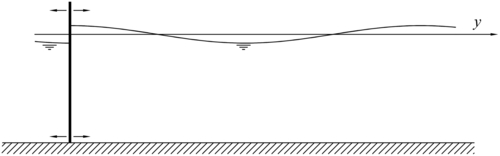
The wavemaker of Fig. 15.3 moves, alternately, rightwards and leftwards at section y = 0 of a waveflume, and yields a given oscillating water discharge

$Q (t) = Q_{\max} \cos (ω t + ε)$ $Q (t) = Q_{\max} \cos (ω t + ε)$

(15.1)

In Section 1.10, we assumed, as a matter of fact, that a wavemaker generates a progressive wave field. A more correct approach would have been assuming that the wavemaker generates a periodic waveform with the most general expression, given that a priori we do not know which is the waveform yielded by the wavemaker. The periodic wave function with the most general form is

$η (y, t) = (α_{1} \cos k y \cos ω t + α_{2} \sin k y \cos ω t + α_{3} \cos k y \sin ω t + α_{4} \sin k y \sin ω t) H$ $η (y, t) = (α_{1} \cos k y \cos ω t + α_{2} \sin k y \cos ω t + α_{3} \cos k y \sin ω t + α_{4} \sin k y \sin ω t) H$

(15.2)

where parameters α₁, α₂, α₃, α₄, and height H are to be determined. The distribution of velocity potential associated with this wave function proves to be

$ϕ (y, z, t) = \frac{g}{ω} (- α_{1} \cos k y \sin ω t - α_{2} \sin k y \sin ω t + α_{3} \cos k y \cos ω t + α_{4} \sin k y \cos ω t) H \frac{\cos h [k (d + z)]}{\cos h (k d)}$ $ϕ (y, z, t) = \frac{g}{ω} (- α_{1} \cos k y \sin ω t - α_{2} \sin k y \sin ω t + α_{3} \cos k y \cos ω t + α_{4} \sin k y \cos ω t) H \frac{\cos h [k (d + z)]}{\cos h (k d)}$

(15.3)

which implies that the water discharge at y = 0, the mean energy flux per unit length, and the mean energy per unit surface are

$Q (t) = (- α_{2} \sin ω t + α_{4} \cos ω t) \frac{ω}{k} H$ $Q (t) = (- α_{2} \sin ω t + α_{4} \cos ω t) \frac{ω}{k} H$

(15.4)

$Φ = 0.50 (α_{1} α_{4} - α_{2} α_{3}) ρ g H^{2} c_{G}$ $Φ = 0.50 (α_{1} α_{4} - α_{2} α_{3}) ρ g H^{2} c_{G}$

(15.5)

$E = 0.25 (α_{1}^{2} + α_{2}^{2} + α_{3}^{2} + α_{4}^{2}) ρ g H^{2}$ $E = 0.25 (α_{1}^{2} + α_{2}^{2} + α_{3}^{2} + α_{4}^{2}) ρ g H^{2}$

(15.6)

where c_G is the group velocity defined by Eqn (1.102). Equating the RHS of Eqn (15.4) to the RHS of Eqn (15.1), we get

$H = \frac{Q_{\max} k}{ω K}$ $H = \frac{Q_{\max} k}{ω K}$

(15.7)

$α_{2} = K \sin (ε), α_{4} = K \cos (ε)$ $α_{2} = K \sin (ε), α_{4} = K \cos (ε)$

(15.8)

where K is an arbitrary constant. Now let us assume that nature chooses the waveform that yields the largest value of the ratio

$C = \frac{Φ}{E c_{G}}$ $C = \frac{Φ}{E c_{G}}$

(15.9)

(later, we shall discuss the base of this assumption). The expression of C proceeds from Eqns (15.5) and (15.6):

$C = \frac{2 (α_{1} α_{4} - α_{2} α_{3})}{α_{1}^{2} + α_{2}^{2} + α_{3}^{2} + α_{4}^{2}}$ $C = \frac{2 (α_{1} α_{4} - α_{2} α_{3})}{α_{1}^{2} + α_{2}^{2} + α_{3}^{2} + α_{4}^{2}}$

(15.10)

C proves to vary between 0 and 1, and the maximum (C = 1) occurs for

$α_{1} = α_{4}, α_{3} = - α_{2}$ $α_{1} = α_{4}, α_{3} = - α_{2}$

(15.11)

With Eqn (15.7) of H and Eqns (15.8) and (15.11) of the α₁, α₂, α₃, and α₄, Eqn (15.2) of η(y, t) becomes

$η (y, t) = Q_{\max} \frac{k}{ω} (\cos ε \cos k y \cos ω t + \sin ε \sin k y \cos ω t - \sin ε \cos k y \sin ω t + \cos ε \sin k y \sin ω t)$ $η (y, t) = Q_{\max} \frac{k}{ω} (\cos ε \cos k y \cos ω t + \sin ε \sin k y \cos ω t - \sin ε \cos k y \sin ω t + \cos ε \sin k y \sin ω t)$

(15.12)

where the unknown constant K cancels. Equation (15.12) can be reduced to

$η (y, t) = Q_{\max} \frac{k}{ω} \cos (k y - ω t - ε)$ $η (y, t) = Q_{\max} \frac{k}{ω} \cos (k y - ω t - ε)$

(15.13)

which represents a progressive wave.

Let us summarize: we have two conclusions.

First conclusion: A wavemaker could generate an infinity of alternative waveforms. We knew that the wavemaker generates a progressive wave. Now we have realized that the progressive wave is the waveform giving the largest value of the dimensionless number C. Maximizing C is as if nature likes reaching the largest energy flux with the lowest storage of energy along the path of this energy flux, and indeed, we may call C the “energy-flux/energy factor.”

Second conclusion: In the problem of the wavemaker that we have re-dealt with, C represents also the ratio between the speed with which the wave motion expands on the waveflume and c_G. Hence, in the infinite set of alternative waveforms that may be generated by the wavemaker, the aforementioned ratio ranges in (0, 1). In other words, the speed with which the wave motion expands on the waveflume can be smaller than or equal to c_G.

We shall assume that both the first conclusion and the second conclusion are valid in general, and in particular that they hold before a U-OWC. Note that, in the case of the U-OWC, the first conclusion will deal with the ratio between the mean energy flux reaching the plant, and the mean energy per unit surface before the plant. Whereas the second conclusion will concern the speed with which the reflected wave energy advances toward the open sea.

15.2.2. The Propagation Speed of Wave Energy

Now let us imagine to place an upright breakwater in the waveflume of Fig. 1.12. The new configuration is shown in Fig. 15.4. After the wave train strikes the breakwater, the wave field before the breakwater is changed

$from 0.5 H \cos (k y - ω t) to H \cos (k y) \cos (ω t)$ $from 0.5 H \cos (k y - ω t) to H \cos (k y) \cos (ω t)$

that is, from the progressive waves to the standing waves. The standing wave field gradually expands seawards with a propagation speed c_R. With the energy equation applied to the control volume of Fig. 15.4, we have

$Φ_{i n} = (E - E_{i n}) c_{R}$ $Φ_{i n} = (E - E_{i n}) c_{R}$

(15.14)

where

E_{i n}

$E_{i n}$

and Φ_in are, respectively, the mean wave energy per unit surface and the mean energy flux per unit length of the incident waves, and

E

$E$

is the mean wave energy per unit surface of the standing wave field. The LHS of Eqn (15.14) represents the average energy entering the control volume per unit time. The RHS represents the average increment of wave energy inside the control volume per unit time. Given that

FIGURE 15.4 After a wave train strikes a wall, a standing wave field expands toward the origin of the channel, with a propagation speed equal to group velocity c_G.

$E_{i n} = \frac{1}{8} ρ g H^{2}$ $E_{i n} = \frac{1}{8} ρ g H^{2}$

(15.15)

$Φ_{i n} = E_{i n} c_{G}$ $Φ_{i n} = E_{i n} c_{G}$

(15.16)

$E = 2 E_{i n}$ $E = 2 E_{i n}$

(15.17)

it follows that

$c_{R} = c_{G}$ $c_{R} = c_{G}$

(15.18)

Finally, let the conventional breakwater be substituted by a breakwater embodying an energy converter (Fig. 15.5). We shall see in the next section that, after the wave train strikes the breakwater, the wave field before the breakwater is changed from

0.5 H \cos (k y - ω t)

$0.5 H \cos (k y - ω t)$

to a form given by Eqn (15.28), that is, from the progressive waves to a complex wave field, which in general will be different both from the progressive waves and from the standing waves. The complex wave field gradually expands seaward with a propagation speed c_R. With the energy equation applied to the control volume of Fig. 15.5, we have

FIGURE 15.5 After a wave train strikes a converter, a wave field given by Eqn (15.28) expands toward the origin of the channel, with a propagation speed c_R.
The ratio χ = c_R/c_G plays the central role in the wave-converter problem.

$(Φ_{i n} - Φ) = (E - E_{i n}) c_{R}$ $(Φ_{i n} - Φ) = (E - E_{i n}) c_{R}$

(15.19)

where

E

$E$

and Φ are, respectively, the mean energy per unit surface and the mean energy flux per unit length of the complex wave field before the breakwater-converter.

Here, we have three inequalities:

$Φ_{i n} - Φ > 0$ $Φ_{i n} - Φ > 0$

(15.20)

$E - E_{i n} > 0$ $E - E_{i n} > 0$

(15.21)

$c_{R} \leq c_{G}$ $c_{R} \leq c_{G}$

(15.22)

The third inequality is based on the assumption made at the end of Section 15.2.1. Indeed, c_R is the propagation speed with which the complex wave motion expands seawards. Inequalities (Eqns (15.20)–(15.22)) are equivalent to

$0 < χ \leq 1$ $0 < χ \leq 1$

(15.23)

$A < 1$ $A < 1$

(15.24)

where χ is the ratio between c_R and c_G, and A is the absorption coefficient:

$χ = \frac{c_{R}}{c_{G}}$ $χ = \frac{c_{R}}{c_{G}}$

(15.25)

$A = \frac{Φ}{Φ_{i n}}$ $A = \frac{Φ}{Φ_{i n}}$

(15.26)

15.3. Interaction between Wave and U-OWC

15.3.1. The Logic Followed: Three Levels of Solution

The problem of the interaction between a wave of given height and period and a U-OWC aims to predict how much of the incident wave energy is absorbed by the plant, and which is the share of the absorbed energy that may be converted into electric power. There are three levels to deal with this problem: First level: it is assumed that the wave field before a breakwater embodying a U-OWC is the same as there would be before a vertical breakwater. Second level: the assumption that the wave field is equal to the wave field before a vertical breakwater is removed; however, the assumption remains that the wave field is periodic in space. Third level: the residual assumption that the wave field be periodic in space is removed. With the second level, the wave height at the breakwater will no longer be 2H, and the wave field will be that of the standing wave we saw in Section 1.7. This is because of the interaction with the U-OWC. Of course, it is possible that the third level will be approached; however, the author believes that the second level is valuable (for the aim of estimating the mean absorbed power) in that the solution obtained is exact under the assumption made. To say it better: were the waves periodic in space, that obtained here below would be the exact linear solution. Specifically, Section 15.3.2 gives the exact linear solution, if c_R (the propagation speed of the reflected wave energy) is equal to the group velocity c_G. Section 15.3.3 gives the exact linear solution, if nature maximizes the energy-flux/energy factor C, as it was suggested in Section 15.2.1.

15.3.2. Second Level: Basic Solution

Let us assume that the wave field before the breakwater-converter is periodic in time and space. Like in Section 15.1, we express this unknown wave field in the more general form for a periodic wave in time and space. This is given by Eqn (15.2), which may be rewritten in the form

$η (y, t) = (β \cos k y \cos (ω t + ε^{'}) + α \sin k y \cos (ω t + ε^{″})) H$ $η (y, t) = (β \cos k y \cos (ω t + ε^{'}) + α \sin k y \cos (ω t + ε^{″})) H$

(15.27)

where β, α, ε′, and ε″ are related to parameters α₁, α₂, α₃, α₄ of Eqn (15.2), and H here will be the height of the incident waves. Since the choice of the time origin is arbitrary, this origin may be shifted so as to rewrite Eqn (15.27) in the form

$η (y, t) = (β \cos k y \cos (ω t) + α \sin k y \cos (ω t + ε)) H$ $η (y, t) = (β \cos k y \cos (ω t) + α \sin k y \cos (ω t + ε)) H$

(15.28)

where ε is equal to the difference ε″ − ε′. Associated to surface elevation Eqn (15.28) is a distribution of velocity potential in the water that is given by

$ϕ (y, z, t) = - g β H ω^{- 1} f (z) \cos (k y) \sin (ω t) - g α H ω^{- 1} f (z) \sin (k y) \sin (ω t + ε)$ $ϕ (y, z, t) = - g β H ω^{- 1} f (z) \cos (k y) \sin (ω t) - g α H ω^{- 1} f (z) \sin (k y) \sin (ω t + ε)$

(15.29)

where

$f (z) = \frac{\cosh [k (d + z)]}{\cosh (k d)}$ $f (z) = \frac{\cosh [k (d + z)]}{\cosh (k d)}$

(15.30)

From the velocity potential, we obtain particle velocities v_y, v_z, and wave pressure Δp in the water. The wave pressure at (y = 0, z = −a) coincides with the Δp(t) on the outer opening of the plant (see Fig. 15.2). From v_y(z, t) at y = 0, we obtain the water discharge Q(t) of the wave at the converter. From v_y(y, z, t) and Δp(y, z, t), we obtain the average wave energy flux Φ. From η(y, t), v_y(y, z, t), and v_z(y, z, t), we obtain the average wave energy

E

$E$

(average with respect to time and space) before the converter. The result is

$Δ p (t) = ρ g β H \cos (ω t) \frac{\cosh [k (d - a)]}{\cosh (k d)}$ $Δ p (t) = ρ g β H \cos (ω t) \frac{\cosh [k (d - a)]}{\cosh (k d)}$

(15.31)

$Q (t) = - g α H ω^{- 1} \tanh (k d) \sin (ω t + ε)$ $Q (t) = - g α H ω^{- 1} \tanh (k d) \sin (ω t + ε)$

(15.32)

$Φ = - 4 α β \sin (ε) Φ_{i n}$ $Φ = - 4 α β \sin (ε) Φ_{i n}$

(15.33)

$E = 2 (α^{2} + β^{2}) E_{i n}$ $E = 2 (α^{2} + β^{2}) E_{i n}$

(15.34)

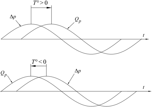
For a given plant and given incident waves, let us fix a tentative value of β, and let us take Δp(t) as input for the calculation of the flow inside the plant, with the sequence described in Section 16.1 (next chapter). The knowledge of the flow inside the plant enables us to obtain Q_p(t) and Φ_p, which are, respectively, the water discharge entering the plant, and the mean energy flux absorbed by the plant (per unit length). As a particular consequence of the knowledge of Q_p(t), we can obtain the time shift T° between Δp(t) and Q_p(t) (see Fig. 15.6). At this point, we can get the three basic equations. The first one says that the phase angle between Δp(t) and Q_p(t) must be equal to the phase angle between Δp(t) and Q(t). The second one says that Φ must be equal to Φ_p. The third one gives the ratio χ between the propagation speed c_R of the reflected wave energy and c_G. These equations are

$ε = - ω T ° - \frac{π}{2}$ $ε = - ω T ° - \frac{π}{2}$

(15.35)

$α = - \frac{Φ_{p}}{4 β \sin (ε) Φ_{i n}}$ $α = - \frac{Φ_{p}}{4 β \sin (ε) Φ_{i n}}$

(15.36)

$χ = \frac{1 + 4 α β \sin (ε)}{2 (α^{2} + β^{2}) - 1}$ $χ = \frac{1 + 4 α β \sin (ε)}{2 (α^{2} + β^{2}) - 1}$

(15.37)

FIGURE 15.6 T° is the time shift between the water discharge entering the plant and the pressure fluctuation at the outer opening of the vertical duct.

As to Eqn (15.35), the phase angle between Δp(t) and Q(t) is equal to –ε − π/2, and the phase angle between Δp(t) and Q_p(t) is the known value ωT°. Equation (15.35) proceeds on equating these phase angles to each other. As to Eqn (15.36), it proceeds straightforwardly from Eqn (15.33). As to Eqn (15.37) of χ, it proceeds from Eqn (15.19) of c_R, with Eqns (15.33) and (15.34) of Φ and

E

$E$

Let us summarize: For a given β, Eqn (15.31) gives Δp(t). Once Δp(t) is known, it is possible to integrate the equations of water–air flow inside the plant (see the next chapter, Section 16.1) and to obtain, in particular, Φ_p and T°. Then, Eqn (15.35) yields ε. With ε being known, Eqn (15.36) yields α. With ε and α being known, Eqn (15.37) yields χ. Hence, one can obtain the functions ε(β), α(β), and χ(β). If we assume that c_R must be equal to c_G (like with an upright breakwater), this assumption closes the problem: the solution will be represented by the β for which χ is equal to 1 (which generally proves to exist and to be unique), and this is the basic solution. Otherwise, if we follow assumption Eqn (15.23) that χ may be between 0 and 1, we may reason as in the next section, which gives the advanced solution.

15.3.3. Second Level: Advanced Solution

With Eqns (15.33) and (15.34) of Φ and

E

$E$

, factor C defined by Eqn (15.9) takes on the form

$C = - \frac{2 α β \sin (ε)}{(α^{2} + β^{2})}$ $C = - \frac{2 α β \sin (ε)}{(α^{2} + β^{2})}$

(15.38)

Besides C, there is a pair of numbers useful for an analysis of the wave field before a breakwater-converter. Of course, one is the absorption coefficient defined either as Φ/Φ_in or Φ_p/Φ_in (given that Φ and Φ_p are equal to each other). Hence, from Eqn (15.36), we have

$A = - 4 α β \sin (ε)$ $A = - 4 α β \sin (ε)$

(15.39)

Then there is the resonance coefficient

$R = 4 \frac{T °}{T}$ $R = 4 \frac{T °}{T}$

(15.40)

where the time shift T° between Q_p(t) and Δp(t) may range in (−T/4, T/4) (with T° in this range, the plant works as an absorber, else it would be a wavemaker). As a consequence, R ranges in (−1, 1): R negative means that the wave period is greater than the eigenperiod; R positive means that the wave period is smaller than the eigenperiod.

FIGURE 15.7 Functions χ(β), A(β), C(β) for: (a) a case in which |R| takes on a relatively small value, and (b) a case of a relatively large |R|.

If R approaches zero (resonance), inequality Eqn (15.23) is satisfied only on a small neighborhood Δβ of some special value β smaller than 1. On this small range of β, χ(β) decreases from 1 to 0, and A approaches 1; C approaches 1.

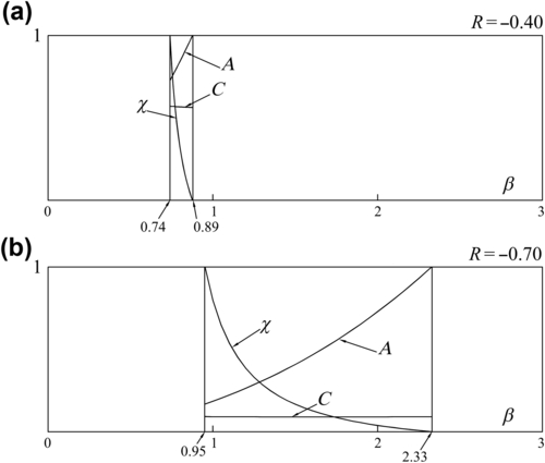
The range of β wherein inequality Eqn (15.23) is satisfied widens as |R| grows, as we may see by comparing Fig. 15.7(a) and (b) to each other. Fig. 15.7(a) shows a case in which R = −0.40 and the inequality Eqn (15.23) prove to be satisfied on the range (0.74 < β < 0.89). Figure 15.7(b) shows a case in which R = −0.70 and the range wherein the inequality Eqn (15.23) is satisfied becomes (0.95 < β < 2.33). Over this range: χ decreases from 1 to 0, and A grows from 0.19 to 1. As to C, it remains essentially constant over the whole range. Therefore, from the reasoning of Section 15.1, nature should choose the solution at random, given that there is not a solution with a value of C greater than that of the other solutions. In this case, there should be the same probability to have any value of β between 0.95 and 2.33. Hence, in a case like that of Fig. 15.7(b), we should expect to find, most probably, a β definitely greater than 1. This expectancy has obtained many confirmations from a small-scale field experiment (SSFE) of 2005. An example is shown in Fig. 15.8 comparing the spectrum of waves at the breakwater-converter to the spectrum of the incident waves. The peak on the first mode, which has an estimated R of about −0.95, is amplified 23 times (!) on passing from the spectrum of the incident waves to the spectrum of the waves at the wall. This superamplification corresponds to a β of about 2.4. (β is equal to the ratio between the RMS surface elevation at the breakwater-converter and the RMS surface elevation that there would be at a conventional upright breakwater.)

FIGURE 15.8 A small-scale field experiment of 2005 on a U-oscillating water column:
the peak of the first mode, which has an estimated R of about −0.95, is amplified 23 times!

The linear theory foresees superamplifications (possibility of very large β) both with large negative R and with large positive R. However, superamplifications require that waves have a very low steepness, otherwise there would be energy losses or wave breaking, and this, practically, limits superamplifications to some long swell with large negative R. In the next chapter we shall see how to address this face of the problem, on a technical-engineering ground.

Here we conclude with the following overall picture: If χ = 1, β is smaller than 1. If β is greater than 1, χ is smaller than 1. If β takes on the total largest value (e.g., β = 2.33 in Fig. 15.7(b)) χ is equal to 0. This means that at the breakwater-converter there is a large wave amplification, which remains locked to the breakwater and cannot expand seawards. The fact that there is no energy advancing seaward implies that the whole incident wave energy is absorbed by the plant, and indeed, we see that the absorption coefficient gets equal to 1.

15.4. Conclusion

The wavemaker boundary value problem for planar wavemakers was given a complete solution thanks, in particular, to Havelock (1929), Hyun (1976), Hudspeth and Chen (1981). This problem aims to obtain the velocity potential yielded by a wavemaker with a given configuration. The area of waveflume close to the wavemaker is focused, wherein waves are not periodic in space because of the presence of evanescent eigenmodes. It is assumed that, far from the wavemaker, the wave is a progressive one. We (Section 15.2.1) wonder whether this last sentence “far from the wavemaker, the wave is a progressive one” must be accepted as a matter of fact or may be explained as a consequence of a general principle (that nature tends to maximize the ratio between Φ and

E

$E$

). Of course, in this context, there is no interest in the evanescent eigenmodes, nor in the configuration of the wavemaker. (Formally, one may shift the origin y = 0 far from the wavemaker; or, at his choice, may think of the configuration of the wavemaker as a curve in such a way that the wave motion can be periodic in space even close to the wavemaker.) Please don't believe that the question at the base of Section 15.2.1 is abstract philosophy. If nature tends to maximize the ratio

Φ / E

$Φ / E$

(which is a velocity), this explains the huge amplification of Fig. 15.8, and let us look with greater optimism at the possibility of industrial exploitation of wave energy. A series of amplifications like that of Fig. 15.8 were found in the SSFE of 2005, illustrated by Boccotti et al. (2007).

..................Content has been hidden....................

You can't read the all page of ebook, please click here login for view all page.

Table of Contents for Chapter 15. Conversion of Wave Energy

Create new playlist

Sign In

Sign Up

Abstract

Keywords

15.1. An Overview of Work Done to Exploit Wave Energy Source

15.2. The Propagation Speed of Wave Energy

15.2.1. Re-analysis of the Problem of a Wavemaker

15.2.2. The Propagation Speed of Wave Energy

15.3. Interaction between Wave and U-OWC

15.3.1. The Logic Followed: Three Levels of Solution

15.3.2. Second Level: Basic Solution

15.3.3. Second Level: Advanced Solution

15.4. Conclusion

Table of Contents for
Chapter 15. Conversion of Wave Energy