Search in book...
Toggle Font Controls
Create new playlist

Name your new playlist

Playlist description (optional)
Sign In

Email address

Password

Forgot Password?

or

Continue with Facebook

Continue with Google
Sign Up

Full Name

Email address

Confirm Email Address

Password

or

Continue with Facebook

Continue with Google

Chapter 13

Calculation of Wave Forces on Gravity Platforms and Submerged Tunnels

Abstract

The general method of Chapter 10 for calculating the largest wave forces on large isolated bodies of arbitrary shape is applied. This method (being based on QD theory and SSFEs) is much simpler than the commonly applied methods using Green's functions, which are summarized in the conclusive notes to the chapter. The first part of the chapter deals with an estimate of the largest wave loads on a gravity offshore platform, in a design sea state. A worked example is given, and a FORTRAN program is supplied that calculates the resultant wave force as a function of time. The second part of the chapter deals with an estimate of the largest wave loads on a submerged tunnel, in a design sea state. Here too, a worked example is given and a FORTRAN program is supplied. This program gives the distributions of the wave force per unit length, at a number of time instants, during the transit of the wave group of the maximum expected wave height.

Keywords

Offshore gravity platform; Quasi-determinism theory (QD); Small-scale field experiment (SSFE); Submerged tunnel; Wave load

13.1. Wave Forces on a Gravity Offshore Platform

What follows is a worked example of an estimate of the wave force on the offshore gravity platform of Fig. 13.1. The data of the design sea state and the estimate of the largest wave height in the lifetime are the same as in the worked example of Chapter 12.

13.1.1. Calculation of the Diffraction Coefficient

For calculating

C_{d_{o}}

$C_{d_{o}}$

of the base, we refer to the circular cylinder of the same area as the base. This has a radius of R = 45 m. Taking

F_{R}

$F_{R}$

= 1.75 for the platform base and

F_{R}

$F_{R}$

= 2.00 for the columns that have an average radius of 8.5 m, with the program of Section 10.7 (with T_p = 16.5 s), we obtain

$platform base : C_{d_{o}} = 1.54$ $platform base : C_{d_{o}} = 1.54$

$columns : C_{d_{o}} ≅ 2.00$ $columns : C_{d_{o}} ≅ 2.00$

FIGURE 13.1 First worked example, Chapter 13: plan and front view (essential scheme) of a hypothesis of support structure of a gravity offshore platform (for details on this kind of structure, see Dawson, 1983).

13.1.2. Calculation of the Wave Force

The FORTRAN program PLAT for a preliminary calculation of the wave force on a gravity offshore platform is listed here below. Point x_o,y_o is taken at the center of the platform. The data of the geometry of the structure are read from the following file:

  File PLATGEO
  140.0 d
  60.0 HTANK (height vertical cylinders)
  110.0 HCOL (height columns)
  20.0 DCYL (diameter vertical cylinders)
  20.0 DCOL1 (greater diameter column)
  14.0 DCOL2 (smaller diameter column)
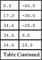
  19 number of vertical cylinders
  coordinates centers cylinders:

0.0	−40.0
17.3	−30.0
34.6	−20.0
34.6	0.0
34.6	20.0
Table Continued

17.3	30.0
0.0	40.0
−17.3	30.0
−34.6	20.0
−34.6	0.0
−34.6	−20.0
−17.3	−30.0
0.0	−20.0
17.3	−10.0
17.3	10.0
0.0	20.0
−17.3	10.0
0.0	−10.0
0.0	0.0

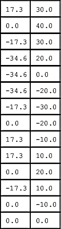
c 3 number of columns
c coordinates centers columns:

0.0	−20.0
17.3	10.0
−17.3	10.0

Loop 100 lets T range in (−1.25T_p,1.25T_p); loop 400 and loop 410 inside loop 100 compute, respectively, the force on the base and the columns, at the given T. Loop 500 inside loop 400 subdivides each of the 19 cylinders of the base into five segments of 12 m in height and computes the wave force on these segments. Loop 510 inside loop 410 subdivides the wet piece (i.e., from z = −80 m to z = η) of a column into 20 segments and computes the wave force on each of these segments. Subroutine QD is called both in the loop 500 and in the loop 510, and provides the

\bar{a_{x}}, \bar{a_{y}}

$\bar{a_{x}}, \bar{a_{y}}$

, which serve for computing the Froude–Krylov force.

A simple way to consider the effect of the 24 interstices among the 19 cylinders of the base is multiplying the force on the 19 cylinders by the ratio (=1.065) between the volume of the base and the volume of the 19 cylinders. The program writes T / T_p, and F_x, F_y in kN.

  PROGRAM PLAT
  CHARACTER∗64 NOMEC
  DIMENSION XCI(20),YCI(20)
  DIMENSION XCO(10),YCO(10)
  COMMON D,HS,H,TP,TST,ALPHA,TETAD,RNP
  COMMON IMAX,JMAX,OMV(300),TETV(150),RKV(300)
  COMMON SOT(300,150)
  NOMEC='PLATGEO'

  .OPEN(UNIT=50,STATUS='OLD',FILE=NOMEC)
  READ(50,∗)D
  READ(50,∗)HTANK
  READ(50,∗)HCOL
  READ(50,∗)DCYL
  READ(50,∗)DCOL1
  READ(50,∗)DCOL2
  READ(50,∗)NCYL
  READ(50,∗)
  DO N=1,NCYL
  READ(50,∗)XCI(N),YCI(N)
  ENDDO
  READ(50,∗)NCOL
  READ(50,∗)
  DO N=1,NCOL
  READ(50,∗)XCO(N),YCO(N)
  ENDDO
 
  NOMEC='FORCE2'
  OPEN(UNIT=60,FILE=NOMEC)
  PG=3.141592
  DPG=2.∗PG
  WRITE(6,∗)'Hs,H'
  READ(5,∗)HS,H
  WRITE(6,∗)'alpha,thetad(degree),np'
  READ(5,∗)ALPHA,TETAD,RNP
  WRITE(6,∗)'zero up-crossing wave -> 1, down-crossing -> -1'
  READ(5,∗)UD
  TETAD=TETAD∗PG/180.
  WRITE(6,∗)'diffraction coefficients base and columns'
  READ(5,∗)CDBA,CDCO
  RO=1.03E3
  DTAU=0.02
  NCALL=0
  CALL QD(NCALL,UD,X,Y,Z,T,VX,VY,VZ,AX,AY,AZ,ETA)
c this call of QD, with NCALL=0, serves to store the directional spectrum.
  NCALL=1
 
  DO 100 J=1,126
c Loop 100: time
  TAU=−1.25+FLOAT(J-1)∗DTAU
  T=TAU∗TP
c FX x-component Froude-Krylov force on the base of the platform
c FY y-component Froude-Krylov force on the base of the platform
  FX=0
  FY=0
  DO 400 N=1,NCYL

c Loop 400: vertical cylinders of the base
    R=DCYL/2
    X=XCI(N)
    Y=YCI(N)
    DS=HTANK/10
    DO 500 I=1,10
c each vertical cylinder is subdivided into 10 pieces;
c loop 500 covers these 10 pieces.
    Z=-D+FLOAT(I-1)∗DS+DS/2
    CALL QD(NCALL,UD,X,Y,Z,T,VX,VY,VZ,AX,AY,AZ,ETA)
    COFI=RO∗PG∗R∗R∗DS
    FX=FX+COFI∗AX
    FY=FY+COFI∗AY
500   CONTINUE
400   CONTINUE
c effect of the interstices among the vertical cylinders
    FBX=FX∗1.065
    FBY=FY∗1.065
c step from Froude-Krylov force to force on the solid body (base)
    FBX=FBX∗CDBA
    FBY=FBY∗CDBA
c conversion from N to kN
    FBX=FBX∗1.E−3
    FBY=FBY∗1.E−3
 
c Here the calculation of the wave force on the base has been completed.
c Now the calculation of the wave force on the columns starts
 
c FX x-component Froude-Krylov force on the columns
c FY y-component Froude-Krylov force on the columns
    FX=0
    FY=0
    DO 410 N=1,NCOL
c Loop 410 columns
    X=XCO(N)
    Y=YCO(N)
    CALL QD(NCALL,UD,X,Y,Z,T,VX,VY,VZ,AX,AY,AZ,ETA)
    HCOLW=d-HTANK
    DS=(HCOLW+ETA)/20
    DO 510 I=1,20
c the wet portion of a column is subdivided into 20 pieces;
c loop 510 covers these 20 pieces
    ZI=FLOAT(I-1)∗DS+DS/2.
    Z=-HCOLW+ZI
    CALL QD(NCALL,UD,X,Y,Z,T,VX,VY,VZ,AX,AY,AZ,ETA)
   DIAM=DCOL1+(DCOL2-DCOL1)∗ZI/HCOL
    R=DIAM/2

  .COFI=RO∗PG∗R∗R∗DS
  FX=FX+COFI∗AX
  FY=FY+COFI∗AY
510  CONTINUE
410  CONTINUE
c step from Froude-Krylov force to force on the solid body (columns)
  FCX=FX∗CDCO
  FCY=FY∗CDCO
c conversion from N to kN
  FCX=FCX∗1.E-3
  FCY=FCY∗1.E-3
c Here the calculation of the wave force on the columns has been completed
c FTX is the x-component of the wave force on the whole structure
c FTY is the y-component of the wave force on the whole structure
  FTX=FBX+FCX
  FTY=FBY+FCY
  WRITE(60,1000)TAU,FTX,FTY
  WRITE(6,1000)TAU,FTX,FTY
1000  FORMAT(2X,F7.2,2X,E12.4,2X,E12.4)
100   CONTINUE
  WRITE(6,∗)
  WRITE(6,∗)'read results on file FORCE2'
  END

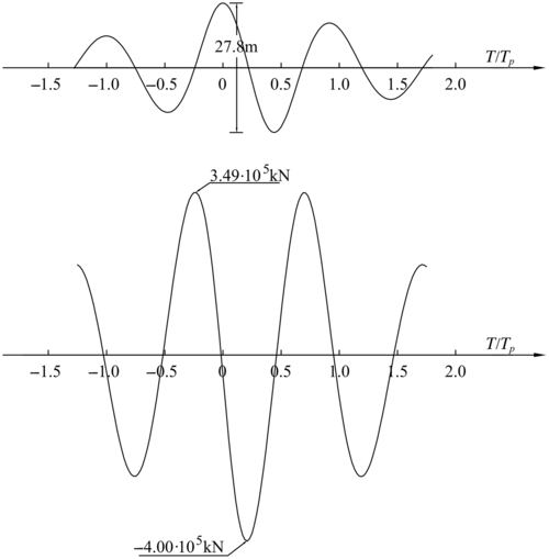
Figure 13.2 shows the horizontal force F_y on the whole structure. Since the angle θ_d between the dominant direction and the y-axis is zero, the wave group moves along the y-axis, so that the horizontal force proves to be parallel to the y-axis (x-component negligible).

13.2. Wave Forces on a Submerged Tunnel

What follows is a worked example of an estimate of the wave force on the submerged tunnel of Fig. 13.3, which has a length of 1000 m and is supported by five piers.

13.2.1. Wave Height and Diffraction Coefficients

Design sea state: H_s = 8 m; duration = 7 h; spectrum: mean JONSWAP, with A = 0.01; dominant direction: θ_d = 0 (orthogonal to the tunnel axis); directional distribution: Mitsuyasu et al. with n_p = 20. For the aim of a preliminary estimate, we resort to the DSSP (see Section 5.6.1). The maximum bending moment in the tunnel occurs if the center of a wave group (like that of Fig. 9.1) strikes a pier. Hence, we must calculate the maximum expected wave height at the five locations of the piers, in the design sea state. Following Section 6.2, this maximum expected wave height at five points (roughly aligned with the wave crests, and with a distance from each other, greater than L_p0/2) may be estimated as the maximum expected wave height at one point in a duration of time five times greater than the actual duration of the sea state. The conclusion turns out to be

$H = 16.8 m, H_{s} = 8.0 m$ $H = 16.8 m, H_{s} = 8.0 m$

FIGURE 13.2 First worked example, Chapter 13: (a) wave group of the maximum expected wave height in the design sea state, (b) horizontal force exerted on the structure (base + columns).

The suggested value of

F_{R}

$F_{R}$

for a submerged tunnel is 2.0, and with this value of

F_{R}

$F_{R}$

and T_p of 12.1s, the FORTRAN program of Section 10.7 gives

$C_{d_{o}} = 1.91$ $C_{d_{o}} = 1.91$

Conservatively,

C_{d_{v}}

$C_{d_{v}}$

will be assumed equal to

C_{d_{o}} .

$C_{d_{o}} .$

FIGURE 13.3 Second worked example, Chapter 13: a hypothesis of submerged tunnel.

13.2.2. Calculation of Wave Force

FORTRAN program TUNN for a preliminary calculation of the wave load on the tunnel is listed below. Loop 100 lets T range in (−1.3T_p, 1.8T_p); loop 400 computes the sectional wave force on a length of tunnel of 600 m that is, more or less, the length of the crest of a wave group at the apex of its development stage, in the design sea state.

Subroutine QD is called in the loop 400, and provides the

\bar{a_{y}}, \bar{a_{z}}

$\bar{a_{y}}, \bar{a_{z}}$

, which serve for computing the Froude–Krylov force. The sectional force f_y and the sectional force f_z are stored, respectively, on FPVY(J,N) and FPVZ(J,N), where J is associated with T, and N is associated with X. Loop 600 writes f_y(X) or f_z(X) in kN/m at the time instants τ = T / T_p in which these forces get a local maximum.

  PROGRAM TUNN
  CHARACTER∗64 NOMEC
  DIMENSION FYV(300),FZV(300),TAUV(300)
  DIMENSION FPYV(300,200),FPZV(300,200)
  COMMON D,HS,H,TP,TST,ALPHA,TETAD,RNP
  COMMON IMAX, JMAX,OMV(300),TETV(150),RKV(300)
  COMMON SOT(300,150)
  NOMEC='LOAD1'
  OPEN(UNIT=60,FILE=NOMEC)
  PG=3.141592
  DPG=2.∗PG
  WRITE(6,∗)'Hs,H'
  READ(5,∗)HS,H
  WRITE(6,∗)'alpha,thetad(degree),np'
  READ(5,∗)ALPHA,TETAD,RNP
  WRITE(6,∗)'zero up-crossing wave -> 1, down-crossing -> -1'
  READ(5,∗)UD
  TETAD=TETAD∗PG/180
  WRITE(6,∗)'horizontal and vertical diffraction coefficients'
  READ(5,∗)CDO,CDV
  RO=1.03E3
  D=125.
c DIAM diameter tunnel
c ZCE z tunnel center
c RLT length of tunnel being considered
  DIAM=25
  R=DIAM/2.
  ZCE=−42.5
  RLT=600.
  DX=RLT/60.
  DTAU=0.02

  .NCALL=0
  CALL QD(NCALL,UD,X,Y,Z,T,VX,VY,VZ,AX,AY,AZ,ETA)
c this call of QD, with NCALL=0, serves to store the directional spectrum
  NCALL=1
 
  DO 100 J=1,156
c Loop 100:time
  TAU=-1.30+FLOAT(J-1)∗DTAU
  WRITE(6,5010)TAU
5010 FORMAT(2X,F7.2)
  TAUV(J)=TAU
  T=TAU∗TP
c FYV(J) resultant wave force (y-component) on the piece
c of tunnel being considered
c FZV(J) resultant wave force (z-component) on the piece
c of tunnel being considered
  FYV(J)=0
  FZV(J)=0
  DO 400 N=1,61
c Loop 400:X (axis tunnel)
  X=-RLT/2.+FLOAT(N-1)∗DX
  Y=0
  Z=ZCE
  CALL QD(NCALL,UD,X,Y,Z,T,VX,VY,VZ,AX,AY,AZ,ETA)
  COFI=RO∗PG∗R∗R
c FPYV(J,N) wave force per unit length (y-component)
c FPZV(J,N) wave force per unit length (z-component)
  FPYV(J,N)=CDO∗RO∗PG∗R∗R∗AY
  FPZV(J,N)=CDV∗RO∗PG∗R∗R∗AZ
c conversion from N to kN
  FPYV(J,N)=1.E-3∗FPYV(J,N)
  FPZV(J,N)=1.E-3∗FPZV(J,N)
  FYV(J)=FYV(J)+FPYV(J,N)∗DX
  FZV(J)=FZV(J)+FPZV(J,N)∗DX
400  CONTINUE
100  CONTINUE
 
  DO 600 J=2,154
c Loop 600: time
c tau=TAUV(J)
c |Fy(tau-dtau)|=AFY1
c |Fy(tau)|=AFY2
c |Fy(tau+dtau)|=AFY3
  AFY1=ABS(FYV(J-1))
  AFY2=ABS(FYV(J))
  AFY3=ABS(FYV(J+1))
  IF(AFY2.GT.AFY1.AND.AFY2.GT.AFY3)THEN

c a local maximum (or minimum) of Fy has been found
  WRITE(60,1000)TAUV(J)
1000  FORMAT(//,6X,'TAU = ',F7.2,4X,'(fy)',/)
  DO 490 N=1,61
c Loop 490:X (axis tunnel)
  X=-RLT/2.+FLOAT(N-1)∗DX
  WRITE(60,1001)X,FPYV(J,N)
1001  FORMAT(2X,F6.0,2X,F6.1)
490  CONTINUE
  ENDIF
c |Fz(tau-dtau)|=AFZ1
c |Fz(tau)|=AFZ2
c |Fz(tau+dtau)|=AFZ3
  AFZ1=ABS(FZV(J-1))
  AFZ2=ABS(FZV(J))
  AFZ3=ABS(FZV(J+1))
  IF(AFZ2.GT.AFZ1.AND.AFZ2.GT.AFZ3)THEN
c a local maximum (or minimum) of Fz has been found
  WRITE(60,1002)TAUV(J)
1002 FORMAT(//,6X,'TAU = ',F7.2,4X,'(fz)',/)
  DO 491 N=1,61
c Loop 491:X (axis tunnel)
  X=-RLT/2.+FLOAT(N-1)∗DX
  WRITE(60,1001)X,FPZV(J,N)
491  CONTINUE
  ENDIF
600  CONTINUE
  WRITE(6,∗)
  WRITE(6,∗)'read results on file LOAD1'
  END

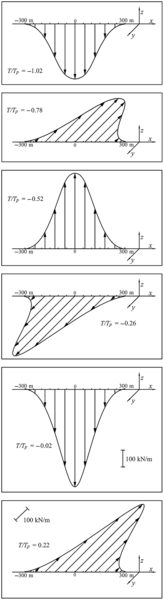
Figure 13.4 shows the local maxima of f_y and f_z. A local maximum of f_y takes place when a zero of the wave group transits over the axis of the tunnel. A local maximum of f_z takes place when a crest or a trough of the wave group transits over the axis of the tunnel.

The SSFE of 1993 at the NOEL on submerged tunnels (Boccotti, 1996) showed a slight asymmetry between positive and negative peaks of the vertical wave force. This is a nonlinearity effect being due to the kinetic term of the wave pressure. This term reduces both the wave pressure on the upper half cylinder and on the lower half. However, the reduction on the upper half is greater than the reduction on the lower half that somewhat enhances the upward (positive) wave force and reduces the downward (negative) force. The kinetic term of the wave pressure can be evaluated from the v_x, v_y, and v_z obtained from the subroutine QD, on the cylinder surface. However, for the sake of simplicity in this example program, this term has been neglected.

FIGURE 13.4 Second worked example, Chapter 13: peaks of the wave load on the tunnel, under the wave group of the maximum expected wave height in the design sea state.

13.3. Conclusion

Wave forces on large bodies under regime of wave diffraction are calculated with the use of Green's functions (John, 1949, 1950; Mei, 1989). The geometry of the structures is described with a large number of panels, which makes the program slower and requires a large PC memory (Chakrabarti, 2005). This is for a single periodic wave. If we would pass to a random sea state, that is, to a summation of harmonic wave components with different frequencies, with the need to cover some large time interval (for getting a satisfactory statistical confidence), the computational problems would become really very great. Chapter 10 eliminates these computational problems, so that the calculation of the wave force on large bodies is reduced to something simple as programs PLAT and TUNN of the present chapter. The gist of Chapter 10 is that there is a simple relationship between the deterministic force exerted by a wave group on a large body and the deterministic force that this wave group exerts on a water mass equivalent to the solid body. In the author's opinion, the progress of the models for calculation of wave load has the following sequence:

step 1 periodic, unidirectional wave,

step 2 long-crested random waves,

step 3 short-crested random waves,

step 4 deterministic mechanics of wave groups.

With “small bodies” (Chapter 12), the QD theory has enabled us to advance from step 3 to step 4; with “large bodies” (present chapter), the QD theory has enabled us to jump from step 1 to step 4.

..................Content has been hidden....................

You can't read the all page of ebook, please click here login for view all page.

Table of Contents for Chapter 13. Calculation of Wave Forces on Gravity Platforms and Submerged Tunnels

Create new playlist

Sign In

Sign Up

Abstract

Keywords

13.1. Wave Forces on a Gravity Offshore Platform

13.1.1. Calculation of the Diffraction Coefficient

13.1.2. Calculation of the Wave Force

13.2. Wave Forces on a Submerged Tunnel

13.2.1. Wave Height and Diffraction Coefficients

13.2.2. Calculation of Wave Force

13.3. Conclusion

Table of Contents for
Chapter 13. Calculation of Wave Forces on Gravity Platforms and Submerged Tunnels