
Chapter 10
QD Theory
Mechanics of Wave Forces on Large Isolated Bodies
Abstract
The propagation speed of pressure head waves in wave groups is reduced to a half at the base and columns of a gravity offshore platform. The same phenomenon is noticed also at submerged tunnels. This explains why the horizontal wave force on large isolated bodies is greater than the Froude–Krylov force. This is the kernel of the chapter, which is based on small-scale field experiments, and exploits the powerful synthesis made possible by the QD theory when applied for analysis-of-time-series data (the chapter shows a pair of figures most evident of this capability to do synthesis). As a consequence, the chapter suggests a general method to calculate the largest wave forces on large isolated bodies, and supplies a FORTRAN program useful for this scope, which will be applied in Chapter 13.
Keywords
Froude–Krylov force; Large isolated bodies; Small-scale field experiment (SSFE); Wave diffraction; Wave force; Wave group10.1. Further Proof that the QD Theory Holds for Arbitrary Configurations of the Solid Boundary
It can be proved that the deterministic velocity potential  satisfies every boundary condition, provided that random velocity potential
  satisfies this boundary condition.
For simplicity, and without loss of generality, we shall assume the solid boundary to be a cylinder (see the reference scheme of Fig. 10.1). Provided that
![]() (10.1)
(10.1)

![]() (10.2)
(10.2)
That is, we aim to prove the following equality:
 (10.3)
If the definition (Eqn (7.9)) of Φ is used, and b/σ2(xo, yo) is canceled from both the LHS and the RHS, the equality to be proved becomes
 (10.4)
To prove this equality, one has to invert the order derivative-average both on the LHS and on the RHS, and use the equality Eqn (10.1).
10.2. Deterministic Pressure Fluctuations on Solid Body
The pressure fluctuation  is related to velocity potential by
![]() (10.5)
(10.5)
![]() (10.6)
(10.6)
and with the definition (Eqn (7.9)) of Φ:
 (10.7)
Finally, on inverting the order derivative with respect to T–average with respect to t, we arrive at
![]() (10.8)
(10.8)
and hence
![]() (10.9)
(10.9)
If a wave crest with a given height b occurs at point xo, yo at time instant to, and b/σ(xo, yo) → ∞, the random wave pressure in space and time, in a neighborhood of xo, yo, will be asymptotically equal to this deterministic function.
If a wave with a given height H occurs at point xo, yo, and H/σ(xo, yo) → ∞, the random wave pressure in space and time, in a neighborhood of xo, yo, will be asymptotically equal to the deterministic function
 (10.10)
which proceeds from the velocity potential (Eqn (8.84)).
These equations of are valid for every point in the water, and thus in particular at the boundary of a solid body with an arbitrary configuration.
10.3. Comparing Wave Pressures on an Isolated Solid Body to the Wave Pressures on an Equivalent Water Body
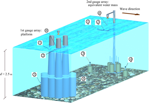
In 1992 and 1993, two small-scale field experiments (SSFEs) were executed in the sea area of the NOEL, for comparing, in real time, wave forces on large isolated bodies to the Froude–Krylov force. The field laboratory of the 1992 experiment is shown in Fig. 10.2. The structure was the 1:50 scale model of an offshore gravity platform of the North Sea.
In the 1:50 scale, the typical sea states consisting of wind seas of about 0.30 m Hs corresponded to full-scale sea states of about 15 m Hs which are realistic design sea states for the North Sea. Wave pressures were recorded by an array of pressure transducers at several points (1, 2, 3, 4) at the boundary of the platform, and the surface elevation was recorded at point 0 above the center of platform's base, by means of an ultrasonic probe. The wave pressures were contemporarily recorded at points (1, 2, 3, 4) with the same spatial configuration of the points at the boundary of the platform, far away where the diffraction effects were negligible. Points (1, 2, 3, 4) may be thought of as points at the boundary of an ideal water platform with the same volume and shape as the solid platform. The surface elevation at point 0 above the center of the base of the equivalent water platform was recorded by a second ultrasonic probe.
1:50 scale model of supporting structure of a gravity offshore platform, and points where wave pressure or surface elevation was measured.
The field laboratory of the 1993 experiment is shown in Fig. 10.3. The structure was the 1:30 scale model of a hypothesis of submerged tunnel across the Messina Straits. Here, the typical 0.30 m Hs corresponded to a full-scale Hs of 9 m, which is consistent with the Hs of the cautious design sea state. Here too, wave pressures were measured at a number of points (5, 12) of the boundary of the solid cylinder, and at the points (5, 12) with the same spatial configuration of the boundary of an ideal water cylinder with the same geometry as the solid cylinder (same radius, same immersion, same water depth, same orientation). The surface elevation was recorded at point 0 above the section of the solid cylinder with points (5, 12). The surface elevation was recorded also at point 0 above the section of the equivalent water cylinder with points (5, 12).

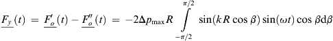
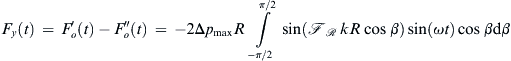
10.4. The Reason the Wave Force on the Solid Body is Greater than the Froude–Krylov Force
Figure 10.4(a) shows the deterministic wave pressure  at the points (i = 1, 2, 3, 4) at the boundary of the solid body of the first experiment. That is, the figure shows the ratio between
![]() (10.11)
(10.11)

(a) Wave pressures at various points of the platform if a wave of given very large height passes at central point 0; (b) wave pressures at various points of the horizontal cylinder if a wave of given very large height passes at point 0 above this cylinder; obtained on applying the algorithm of the QD theory with time series data.
![]() (10.12)
(10.12)
Equation (10.11) is the same as Eqn (10.10) for the special case that point xo, yo is point 0 and point xo + X, yo + Y, z is point i. Figure 10.4(b) shows the deterministic wave pressure at the points (i = 5, 6,…,12) at the boundary of the solid body of the second experiment. Figure 10.5 is the same as Fig. 10.4, with the only difference that the water body is considered in place of the solid body, and hence, the time series data of (0, 1, 2,…) are used instead of (0, 1, 2,…).

(a) Wave pressures at various points of the water body equivalent to the platform if a wave of given very large height passes at central point 0; (b) wave pressures at various points of the water cylinder equivalent to the solid cylinder if a wave of given very large height passes at point 0 above this water cylinder, obtained on applying the algorithm of the QD theory with time series data.
On comparing Fig. 10.5 to Fig. 10.4, we see that the phase angle between a pair of points at the solid body is nearly twice the phase angle between the same pair of points at the water body. For example, the time shift between point 1 and point 2 at the column of the platform is 0.134 s, whereas the time shift between the same pair of points at the water body is 0.067 s.
Typically, a larger phase angle implies a larger pressure difference between the wave beaten half of a cylinder and the sheltered half, and this is the essential reason why the horizontal force on the solid cylinder is greater than the horizontal force on the water cylinder.
As to the effect of the amplitude of the pressure fluctuations, let us consider the RMS pressure fluctuation σi at various points. As to points like 3, 4 of the platform base and 3, 4 of the equivalent water body, σi is the same in 3, 4, 3, 4. Nearly the same holds also for points 1, 2, 1, 2 of the column and of its equivalent water body.
The σi at the tunnel are shown in Fig. 10.6. We see that, from the water cylinder to the solid cylinder, the σi grows on the upper half, and is decreased on the lower half. Of course, this is the reason the amplitude of the vertical wave force on the tunnel is greater than the amplitude of the vertical Froude–Krylov force.
On the opposite, we see that the average σi either on the wave-beaten half-cylinder or on the sheltered half cylinder has only a small change from the water cylinder to the solid cylinder. This implies that the amplification of the horizontal wave force from the horizontal water cylinder to the horizontal solid cylinder depends essentially on the reduction of the propagation speed of the pressure head waves at the solid cylinder, just as it happens for the vertical cylinder.
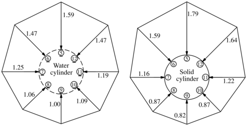
The polar diagram represents the average ratio  in the whole set of records. Here, i denotes the location of the ith measurement point. The diagram on the left is relevant to the water cylinder. The diagram on the right is relevant to the solid cylinder.
in the whole set of records. Here, i denotes the location of the ith measurement point. The diagram on the left is relevant to the water cylinder. The diagram on the right is relevant to the solid cylinder.10.5. Comparing Wave Force on an Isolated Solid Body to the Froude–Krylov Force
The y-z components of the sectional wave force on the tunnel were obtained by means of
![]() (10.13)
(10.13)
![]() (10.14)
(10.14)
where
![]() (10.15)
(10.15)
![]() (10.16)
(10.16)
![]() (10.17)
(10.17)
Equations of the form
![]() (10.18)
(10.18)
![]() (10.19)
(10.19)
![]() (10.20)
(10.20)
![]() (10.21)
(10.21)
may be used for calculating the random (actual) wave force and the deterministic wave force on a solid body with an arbitrary configuration. With Eqn (10.11) in Eqns (10.20) and (10.21), we get
![]() (10.22)
(10.22)
![]() (10.23)
(10.23)
Finally, on inverting the order ∑ with respect to i–average with respect to t, we arrive at
![]() (10.24)
(10.24)
![]() (10.25)
(10.25)
which is the relationship between the deterministic wave force and the random (actual) wave force.
A property that emerged, on the whole, from the two SSFEs was the following:
![]() (10.26)
(10.26)
![]() (10.27)
(10.27)
where
and  and
and  are, respectively, the diffraction coefficient of the horizontal wave force, and the diffraction coefficient of the vertical wave force:
![]() (10.28)
(10.28)
![]() (10.29)
(10.29)
Both the experiments were concerned with wind seas, and y was close to the dominant wave direction; moreover, in the second experiment, y was also the orthogonal to the horizontal cylinder. A proof of properties (Eqns (10.28) and (10.29)) is shown in Fig. 10.7.

Solid line: deterministic wave force on the tunnel. Dashed line: product of the diffraction coefficient and the deterministic wave force on the equivalent water cylinder. Deterministic forces obtained on applying the algorithm of the QD theory with the time series data.
10.6. A General Model for Calculating the Diffraction Coefficient of Wave Forces
We refer to the sketch of Fig. 10.8 showing the cross-section of a vertical water cylinder. Let us think of the cylinder as being subjected to two horizontal wave forces  and
and  , the first one acting on the left half-cylinder (the wave beaten half) and the second one acting on the right half-cylinder (the sheltered half).
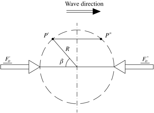
These forces are
 (10.30)
 (10.31)
where Δpmax is the amplitude of the pressure fluctuation at the given depth. On passing from the water cylinder to the solid cylinder, what changes is only the phase angle: the phase angle of a pair of points like P′, P″ grows
![]()
and we have seen that the phase speed reduction factor  is about 2.
Therefore, the forces  and
and  on the two halves of the solid cylinder are
 (10.32)
 (10.33)
 (10.34)
 (10.35)
and hence
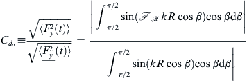 (10.36)
The following suggestions proceed from the experience of the two SSFEs of 1992 and 1993:
1. Equation (10.36) may be applied also with horizontal cylinders (provided that the wave attack is orthogonal to the cylinder axis);
3. may be taken as 1.75 for a base of a gravity platform, and 2 for columns of a gravity platform and tunnels.
As to for submerged tunnels, it proved to be about 10% smaller than . Equation (10.36) and the suggestions enable one to do a quick estimate of the diffraction coefficient. However, we recommend also doing a precise estimate. Then, with the same gauge array suitable for obtaining and/or one may also verify the crucial conclusions (Eqns (10.26) and (10.27)).
10.7. Overall Synthesis
The conclusion of this chapter consists of Eqns (10.26), (10.27) and (10.36). Equations (10.26) and (10.27) say that extreme wave loads on large isolated bodies are equal to the Froude–Krylov force multiplied by the diffraction coefficient. Equation (10.36) may be used for calculating this coefficient. Equation (10.36) is based on the fact that the horizontal wave force on a large isolated body is greater than the horizontal Froude–Krylov force only because of a reduction of the propagation speed of pressure head waves at the solid body. Hereafter is a FORTRAN program to calculate by means of Eqn (10.36).
  PROGRAM CODIF
  PG=3.141592
  DPG=2.∗PG
  G=9.8
  WRITE(6,∗)'d,diam,Tp'
  READ(5,∗)D,DIAM,TP
  WRITE(6,∗)'FR'
  READ(5,∗)FR
  R=DIAM/2
  RLP0=(G/DPG)∗TP∗TP
c RLP0=dominant wavelength on deep water
  RLP=RLP0
 75 RL=RLP0∗TANH(DPG∗D/RLP)
  TEST=ABS(RL-RLP)/RL
  RLP=RL
  IF(TEST.GT.1.E−4)GO TO 75
c RL=dominant wavelength on water depth d
  RK=DPG/RL
  DBETA=PG/200.
  .BETA1=-PG/2.
  BETA2=PG/2.
  BETA=BETA1-DBETA/2.
c RINTNUM=integral numerator RHS Eqn (10.36)
c RINTDEN=integral denominator RHS Eqn (10.36)
  RINTNUM=0
  RINTDEN=0
c Loop 90: integrals on the RHS of Eqn (10.36)
 90 BETA=BETA+DBETA
  IF(BETA.GT.BETA2)GO TO 91
  ARG=FR∗RK∗R∗COS(BETA)
  RINTNUM=RINTNUM+SIN(ARG)∗COS(BETA)
  ARG=RK∗R∗COS(BETA)
  RINTDEN=RINTDEN+SIN(ARG)∗COS(BETA)
  GO TO 90
 91 CONTINUE
  CDO=ABS(RINTNUM)/ABS(RINTDEN)
  WRITE(6,1000)CDO
1000 FORMAT(2x,'Cdo=',F7.3)
  END
10.8. Conclusion
The SSFEs of 1992 and 1993 were described, respectively, by the author (1995) and (1996). These were unusual experiments, not only for their nature of SSFEs. For the first time, as far as is known, there was a real-time comparison between measured wave force and measured Froude-Krylov force. Then, the QD theory was exploited to evidence the relationship between actual wave forces and Froude–Krylov forces. In particular, it exploited the fact that the  obtained through QD Eqn (10.11) always looks regular, as in Figs 10.4 and 10.5, even though it is obtained from random time-series data of surface elevation and wave pressures. Recently, some experiments to verify the QD theory have been performed in a waveflume (Petrova et al., 2011). Notwithstanding their peculiarity, the SSFEs of 1992, 1993 could also be verified in a waveflume at one's choice.
..................Content has been hidden....................
You can't read the all page of ebook, please click here login for view all page.