
5.1 Fundamentals of Video Coding
With the advancement of 2D video compression technology, end users can experience better visual quality at much lower bit rate. To take advantage of the successful development from existing 2D video coding tools and their fast deployment in the marketplace, the 3D video codecs are often built based on the popular 2D video codecs, especially with consideration of the availability of hardware platforms. The mature state-of-the-art video codec, H.264 (MPEG-4 Part 10, Advanced Video Coding (AVC)) [1], has often been selected as a fundamental building block and code base to construct advanced 3D video codecs. Before we introduce the 3D video codecs, we first overview the fundamentals of 2D video coding and the important components adopted in H.264. A short overview of the next generation video codec, high efficiency video coding (HEVC), will be presented at the end of this section.
The modern consumer video codecs often deploy lossy compression methods to achieve higher compression efficiency, so the reconstructed pixels in each frame may not be bit-to-bit accurate when compared to the original video data. The degradation of the perceived video quality is related to the encoded bit rate: a stream with higher bit rate can provide better visual quality and vice versa. The key methodologies adopted in lossy video compression are prediction, transform, quantization, and entropy coding technologies. The concept of a prediction process consists of two coding paths: the reconstruction path and the prediction path. The reconstruction path will decode the already encoded elements and reconstruct the elements to serve as the prediction base. The prediction path is: predict a raw unencoded element from prediction bases, which are normally already encoded elements from the reconstruction path; compute the difference between the predicted value and the raw unencoded value as the prediction error (residual); and encode the prediction error. Note that including the reconstruction path in the prediction process can reduce the overhead for transmitting the initial prediction base. A better prediction can result in smaller prediction error (residual) and thus a potentially smaller number of bits to encode the prediction error. The reconstruction path is presented in both the encoder and the decoder; and the prediction path only appears at the encoder. The transform process is to convert data from one domain to another. It is often observed that the energy in the pixel domain is widely spread among most pixels, which leads to the need to encode almost all pixels into the compressed bit stream. The main purpose of transform is to compact the energy from the original pixel domain to the new domain such that we have as few significant coefficients as possible. Having the transform process, we only need to encode those important coefficients to reduce the required number of bits. The quantization process can be deployed during the encoding process to further reduce the required bits since it can reduce the size of the codeword. However, the quantization process loses information and introduces quantization distortion. The quantization step size has the role of trading off between bit rate and video quality. Entropy coding is a process for compressing data as much as possible in a lossless way. The goal of this lossless compression is to approach the entropy of the coding elements as closely as possible.
Note that modern codecs often adopt block based coding methodology by partitioning one image into multiple nonoverlapped small blocks. The block based processing can help the coding tools to explore the local characteristics of the video data. For color video compression, the video codec often converts the common capture/display three-primary-color space RGB, which represent the red, green, and blue in each color channel, to coding color space YCbCr. The Y component in YCbCr color space represents the luminance information and Cb/Cr represents the chrominance information. As human eyes are more sensitive to the luminance than the chrominance, the Cb and Cr components can be further spatially downsampled to reduce the bit rate.
To be more specific, we show the encoder architecture and the decoder architecture for H.264 in Figure 5.1a, and Figure 5.1b, respectively. As revealed from the figure, the functionality of the encoder is a superset of the decoder. The decoder only consists of the reconstruction path to obtain the decoded signal. The encoder consists of both the prediction path and the reconstruction path. The fundamental coding tools adopted in H.264 consist of (1) intra-frame prediction, (2) inter-frame prediction, (3) de-correlation transform coding, (4) quantization, (5) entropy coding, and (6) deblocking filter.
The intra-prediction process is to explore the spatial redundancy in each individual video frame. It is often observed that neighboring blocks exhibit similar content. For example, an edge may go across multiple blocks; and neighboring blocks may have similar edge direction and/or analogous texture on both sides, separated by the edge. Instead of directly encoding each block, one could deploy the spatial prediction from already decoded pixels in the neighboring blocks to predict the pixels in the current block. Depending on the color component, namely, luma or chroma, there are different block sizes supported in the H.264 standard such that the optimal block size can be chosen adaptively according to local characteristics. The block size for luma intra-prediction defined in H.264 has three different width and height dimensions: 4 × 4, 8 × 8, or 16 × 16. Since an edge in an image may point in a variety of directions, or blocks may contain directional texture, the spatial prediction accuracy depends on the direction of the edges and/or texture. Multiple prediction directions for different block sizes are defined in H.264. As an example, for a 4 × 4 block there are nine different prediction methods that we can choose, namely, vertical prediction, horizontal prediction, DC prediction, diagonal down-left prediction, diagonal down-right prediction, vertical-right prediction, horizontal down prediction, vertical-left prediction, and horizontal-up prediction. The intra-prediction process is illustrated in Figure 5.2. Each rectangle box represents one pixel and the white and gray boxes represent the reconstructed (after encoding and decoding) pixels in the neighboring blocks and the current to-be-encoded pixels in the current block, respectively. Pixels A, B, C, D, E, F, G, H are from top neighbor (TN) blocks; pixel I, J, K, L are from left neighbor (LN) block; and pixel M is from top-left neighbor block (TLN). The dotted line with arrow represents the prediction direction indicating that the pixels along the dotted line in the current block are predicted from the neighbor block's pixel(s) associated with the dotted line. For example, in the vertical prediction, the first column of the pixel in the current block is predicted using pixel A. When the horizontal prediction method is used, the first row of the block is predicted from pixel I. Depending on the location and coding mode surrounding the current block, some neighbor blocks may not be available. The actual prediction process needs to be dynamically readjusted to address the different availability of neighbor blocks. Note that this adaptive prediction is conducted in both the encoder and the decoder through the reconstruction path to ensure the correct usage of neighboring information to avoid wrong operations. For the luma intra 8 × 8, there are also nine different prediction methods similar to the 4 × 4 block size defined in H.264 spec. Besides the block size, the major difference between intra 8 × 8 and intra 4 × 4 is that the pixels in the neighbor blocks are low-pass filtered first and then served as the predictor for intra 8 × 8 case. This low-pass filtering process can help to alleviate the high frequency noise and improve the prediction accuracy and thus overall encoding performance. For the luma intra-prediction based on 16 × 16 block, there are four different prediction methods: vertical prediction, horizontal prediction, DC prediction, and plane prediction. The block size for chroma intra-prediction defined in H.264 only supports dimension with 8 × 8. There are four prediction modes for chroma intra-prediction and the prediction modes are the same as luma intra 16 × 16 modes.
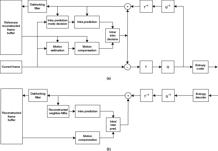
Figure 5.1 (a) Architecture of H.264 encoder. (b) Architecture of H.264 decoder.
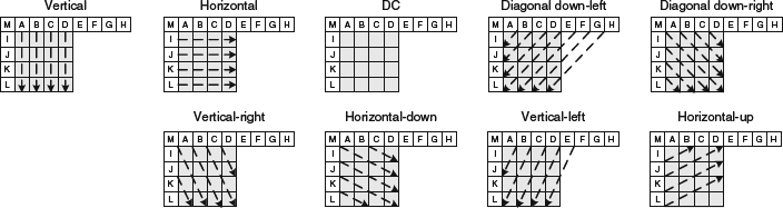
Figure 5.2 Nine different prediction methods for 4 × 4 block in H.264.
With the rich set of multiple prediction sizes and directions, the encoder has more freedom to decide which prediction block size and prediction direction to apply with the consideration of rate and distortion. After having the predicted pixels for each block, we will take the difference between the original pixels and the predicted pixels to output the residual. The residual will be sent to the next stage known as the transform process.
Besides the spatial intra-prediction, it is often observed that consecutive video frames have similar content, and each object has a certain level of displacement from frame to frame. This kind of temporal redundancy can be explored by finding the object movement between neighboring frames along the time domain. More precisely, the modern video codec will partition the current video frame into multiple fixed-size blocks, and try to find the best matched block from the existing decoded frames (as reference frame) via a motion estimation process. We show the motion estimation process in Figure 5.3. In this example, for the rectangular block with line pattern in the current video frame, one can find a “best matched” block with the same dimension in the reference. The relative displacement between the original block and the best matched block is called the motion vector.
The criteria for “best matched” block depend on the optimization objectives defined in the encoder. A commonly adopted measurement is the mean of absolute difference (MAD) among all pixels between the current block in current frame, denoted as Bc, and the candidate block in the reference frame, denoted as Br.
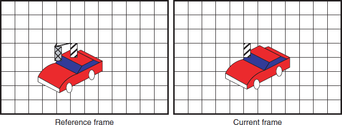
Figure 5.3 Illustration of motion estimation.

where A is the set of coordinates in the current block, (mx, my) is the motion vector with magnitude mx in the horizontal direction and my in the vertical direction. By searching all possible motion vectors, one can choose the optimal motion vector to minimize the MAD. Note that the encoding motion vector also requires a certain number of bits. Besides, the MAD measurement only presents the energy of prediction error and does not indicate the required number of bits to encode the prediction error. A more advanced method from rate-distortion optimization perspective will be discussed in Chapter 10.
After finding the motion vectors, for each to-be-encoded block, we will perform motion compensation with the aid of motion vectors. The best-matched block from the reference frame will be placed at the current block to serve as the predictor. After calculating the difference between the current undistorted block and the motion compensated predictor, we send this residual to the next stage for transform coding. Note that there are several advanced methods to improve the performance of motion estimation; such as:
- subpixel motion estimation: due to the fixed sampling grid on the camera sensors, the actual movement of an object may not appear exactly on the integer grid. Instead, the true motion vectors may be located in the fractional pixel. In this case, interpolation from existing reconstructed pixels are needed to obtain the upsampled reference pixels,
- multiple reference frames: an object may appear in multiple reference frames. Since the movement and lighting condition may change from frame to frame, best motion vectors may be found by allowing search among several decoded reference frames,
- variable block size: having fixed the size of block in the motion estimation/motion compensation process we may not be able to address the different characteristics locally. Allowing different block size can facilitate minimizing the residual for different size of object,
- weighted prediction: multiple motion predicted values from multiple matched blocks can be fused via weighted prediction to achieve better prediction.
The residual that is generated either from the spatial intra-prediction or the temporal inter-prediction will be transformed via block based 2D discrete cosine transform (DCT) to de-correlate the correlation exhibited in the pixel domain. As the coding gain via the DCT transform has been shown as the closest one to the theoretical upper bound, KLT, among all other transforms, under the assumption with first order Markov process in the pixel domain. After 2D DCT, the pixels in each block are represented by DCT coefficients, in which each 2D DCT coefficient indicates the magnitude of the corresponding spatial frequency in both horizontal and vertical directions. For most nature images, there is a larger amount of energy shown in the low spatial frequency, such as smooth areas, and less at high spatial frequency, such as sharper edges. By applying DCT, the energy of each block in the DCT domain will be compacted into a few low frequency DCT coefficients. This process will facilitate the encoding tradeoff between rate and distortion, that is, we may want to preserve more low frequency coefficient information than high frequency ones when the bit budget is limited. The 2D-DCT transform for an input N × N block f(x, y) in the pixel domain to output F(u, v) in the DCT domain can be performed as follows:

with u, v, x, and y being 0,1, 2, …, N − 1 and C(u) and C(v) defined as:
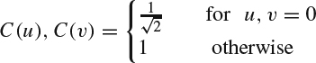
In the older standards, such as MPEG-2, the DCT transform is conducted in the floating point fashion, which might result in slightly different output at the decoder since different platforms and hardware have different implementations for floating point calculation. To achieve bit-to-bit accuracy among all decoders, H.264 adopts an integer DCT transform. Two different DCT transform block sizes, 4 × 4 and 8 × 8, are standardized in the H.264 spec, which provides freedom for the encoder to select according to the content complexity. For intra 4 × 4 coding, a Hardamard transform is again applied on top of all the collected 16 DC DCT coefficients from a 16 × 16 block for further bit rate reduction.
The quantization process will take place after the DCT transform to quantize each of the DCT coefficients. The concept of quantization is to use a smaller set of codewords to approximately represent a larger set of codewords. Consequently, the de-quantized signal is a coarser representation of the original signal. A general form for quantizing a signal x with quantization step size, QS, is performed as follows:
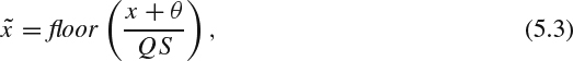
where θ is the rounding offset. The de-quantization process to obtain the reconstructed value, ![]() , is conducted as follows:
, is conducted as follows:
Note that the quantization process is the only component to lose information in the whole video encoding process. Quantization also plays an important role in controlling the bit rate and the quality. With a larger quantization step size, the quantized coefficients have smaller magnitude, thus the encoder can use fewer bits encoding the quantized values. On the other hand, with smaller quantization step size, the coefficients have larger magnitude, resulting in a higher bit rate. To allow a fine granularity of quantization step size for better visual quality and bit rate control, the H.264 standard defines a lookup table to map the quantization parameter (QP) specified from the bit stream syntax to the actual quantization step size.
In H.264, the DCT transform and the quantization are merged into the one process to reduce the computational complexity. It is observed that the magnitude of quantized DCT coefficients in both high horizontal and/or high vertical frequency is smaller than the low frequency coefficients, or close to zero. Instead of directly encoding those quantized coefficients in a raster scan order, having those coefficients reordered according to the magnitude in a descending way can further improve the coding efficiency in the next encoding stage. After this joint process, the encoding order of the quantized DCT coefficients will be reordered in a zigzag way such that the low frequency DCT coefficients are scanned and encoded first and high frequency coefficients are processed later.
| Symbol | Codeword |
| 0 | 1 |
| 1 | 010 |
| 2 | 011 |
| 3 | 00100 |
| 4 | 00101 |
| 5 | 00110 |
| 6 | 00111 |
| 7 | 0001000 |
| 8 | 0001001 |
The final stage of the codec is the entropy coding. The main purpose of entropy coding is to explore the statistical redundancy among the coding symbols constructed from the quantized DCT coefficients. The principle of entropy coding is to assign fewer codewords to the symbols appeared more frequently and longer codewords for symbols occurred less frequently. In this way, we can achieve statistical gain. There are three different entropy coding approaches adopted in H.264 codec: Exp-Golomb coding, context adaptive variable length coding (CAVLC), and context adaptive binary arithmetic coding (CABAC) [2]:
- Exp-Golomb coding: The Exp-Golomb code is designed to optimize the statistical gain when the symbols have geometric distribution. A group of video coding symbols are first mapped to a list of code numbers via a table. Note that different type of coding elements may have different mapping tables and symbols with sign (+/−) can also be encoded by Exp-Golomb code through mapping. The mapping process should ensure that the most frequently occurring symbols are assigned with the smallest value of code numbers; and the least frequently occurring symbols are assigned with the largest code numbers. The Exp-Golomb coding will encode each code number to construct the encoded bit stream with the following structure:
[n bits of 0] [1] [n bits of INFO]
where
n = floor(log2(code number + 1))
INFO = code number +1 − 2n
We show one example in Table 5.1.
The Exp-Golomb code is used universally for almost all symbols in H.264 except for the transform coefficients.
- CAVLC: CAVLC is based on Huffman coding to explore the symbols' distribution, especially when the distribution is not the geometric distribution used in Exp-Golomb code. The Huffman coding is to build a coding/decoding Huffman code tree which best approximates the entropy via an integer number of bits representation. The construction of a Huffman code tree is illustrated in Figure 5.4. Assume that we have four coding symbols, s0, s1, s2, and s3 and the occurrence of each symbol has probability 0.25, 0.55, 0.15, and 0.05, respectively. The tree building process is to merge two nodes with the lowest probability together to form a new parent node and assign the probability of this new node as the sum of the probability from these two child nodes. This process is repeated until we reach the root. Taking Figure 5.4 as an example, in the first step, node s2 and s3 have the lowest probability and we will merge them as node A and assign its probability as 0.2. In the next step, node s0 and node A have the lowest probability, 0.25 and 0.2, respectively. We will merge s0 and A to form node B with a new merged probability 0.45. The last stage is to merge node s1 and B to construct node C. The codeword for each symbol is assigned by tracking back the Huffman tree from the root to the leaf. Note that Huffman coding can be improved by grouping several different symbols together as vector Huffman coding to achieve finer probability representation so as to improve the coding efficiency. In addition, H.264 adopts the context adaptive approach to choose a different Huffman table with different probability distribution with consideration of the neighbor's context.
- CABAC: The major disadvantage of Huffman coding is that it cannot closely approach the entropy bound since each symbol needs at least one integer bit. The arithmetic coding solution is to modify the concept of the vector Huffman coding method but to convert a variable number of symbols into a variable length codeword. The real implementation of arithmetic coding is to represent a sequence of symbols by an interval in the number line from zero to one. Note that the basic form of arithmetic coding uses floating point operation to construct the interval in the number line and needs multiplication operations. Fast binary arithmetic coding with probability update via lookup table can enable multiplication-free calculation to reduce the computation complexity. To utilize the fast binary arithmetic coding, an encoding symbol needs to be binarized through a binarization process such that a symbol is represented by multiple binary bins according to the local context. The binary arithmetic coding operates on those binary bins to output the compressed bit streams.
As those codewords have variable length, any bit error introduced into the stream may lead to different symbols during the decoding process, as no synchronization signal is present to help.
As the quantization is conducted on the DCT coefficients, the reconstructed video often shows blocky artifacts along the boundaries of blocks. For video codecs developed earlier than H.264, those artifacts are often alleviated by video post-processing, which is not mandatory in the codec design. In H.264, the deblocking process is included as an in-loop process to equip the codec with the ability to reduce the blocky artifacts through FIR filtering across block boundaries. Note that the deblocking process can improve the subjective visual quality, but often shows little gain in the objective metric. To avoid deblocking a true edge and apply different strengths of deblocking filtering adaptively, there are multiple criteria and filtering rules defined in the spec. Since those operations involves lots of “if-else” conditions, which are difficult to implement through parallel computing, the computation complexity of the deblocking process takes around at least 30% of overall decoding computation even in a highly optimized software [3].
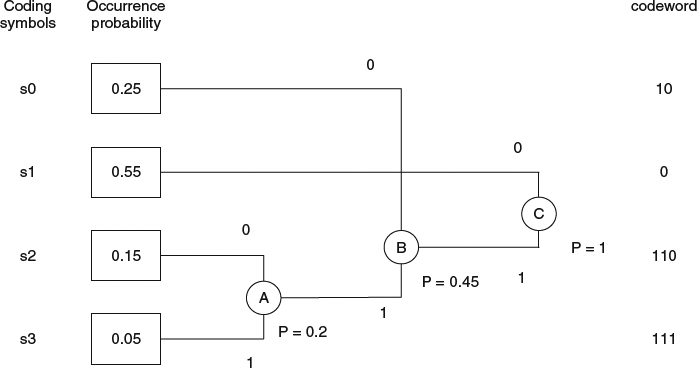
Figure 5.4 Construction of Huffman code tree.
In Figure 5.5, we show the coding hierarchy of H.264 codec. The basic coding unit (CU) in the video codec is called the macroblock (MB), which has dimension 16 × 16 (the chroma has different dimension depending on the chroma sampling format). Each MB is further partitioned into smaller blocks. The dimension of those smaller blocks can be 16 × 16, 16 × 8, 8 × 16, or 8 × 8. For an 8 × 8 block, we can further partition it into sub-blocks of size 8 × 8, 4 × 8, 8 × 4, and 4 × 4. For each block or sub-block, we can choose a different prediction method to achieve our targeted R-D performance. The upper hierarchy on top of the MB is the slice, which defines a global attribute, such as allowing intra-prediction only (I-slice), or adding one more temporal prediction (P-slice), or having intra, single, and bi-prediction (B-slice). A slice can be independently decoded without information from any other slices. This self-contained property makes the bit stream more robust to bit error during the transmission. Each video frame can contain multiple slices, which increases the robustness of the bit stream and enables the possibility of parallel decoding for real-time playback. A frame can be an I (intra-) frame if it contains only I-slice(s), P-frame if it contains both I and P slices, and B-frame if it contains I, P, and B slices, as shown in Figure 5.5. All pictures between two I-frames are grouped together and called a group of pictures (GOP). Note that in H.264, a predictive frame can have multiple reference frames which are stored in the reference picture buffer, and possibly the reference frames' time stamp can be before intra-coded frames. To allow random access to a particular scene, an instantaneous decoder refresh (IDR) coded picture is defined in H.264 to clear the data stored in the reference picture buffer. With IDR, all following received slices can be decoded without reference to any frames decoded prior to the IDR picture.
In the older video standards, a B-frame can only use I and P-frames as reference frames to find the best matched blocks. H.264 allows B-frames to serve as reference frames. This increased freedom enables the encoder to find better matched blocks in the finer scale time domain for more bit rate saving. In addition, this new freedom can construct hierarchical prediction [4]. As shown in Figure 5.6, the first level of hierarchical B-frame, denoted as B0, is bi-predicted from two nearby I0/P0 frames. After obtaining the reconstructed B0, we can further use the first level B-frames for motion references. The second level of the hierarchical B-frames, denoted as B1, is bi-predicted from two nearby I0/P0 frames and the first level hierarchical B-frames. The third level of hierarchical B-frames can be constructed in a similar way. The advantages of using hierarchical B-frames include better coding efficiency and temporal scalability support. The penalty brought by this method is the longer decoding delay and larger memory buffer.
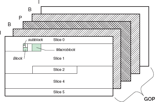
Figure 5.5 Syntax and coding hierarchy.
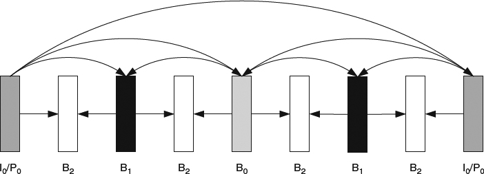
Figure 5.6 Coding structure for hierarchical B-frame.
For the video streaming applications, owing to the varying bandwidth in the transmission channel, it is often desired to have an adaptive streaming design so that the bit rate of the encoded video streams can fit into the allocated bandwidth dynamically. For the online encoded applications with feedback from the receiver, real-time encoding can adjust the coding parameters to change the bit rate. However, for the off-line encoded stored video, the transmitter side needs to prepare multiple versions of the same content and each one is encoded at a different target bit rate. According to the allocated bandwidth, the transmitter will switch to the version with the highest possible bit rate through the current channel such that the end users will experience smooth playback with less viewing disturbance. Owing to the motion compensation across video frames, the switch points are only allowed at the IDR pictures to avoid drifting artifacts. Since the time interval between two nearby IDR pictures is often long, to reduce the coding penalty brought by intra coding, the stream switch time is long and the application cannot respond to the fast varying bandwidth in a timely manner. On this regard, switching P (SP) and switching I (SI) slices are introduced into the H.264 spec [5].
The usage of SP-frame in the bit stream switching from stream 0 to stream 1 is illustrated in Figure 5.7. There are two types of SP-frame: primary and the secondary. The primary SP-frame is encoded in each bit stream and serves as a switching point. Denote the frame index of the desired switching point as n. Frame SP0,n and SP1,n are the primary SP-frames. The secondary SP-frame, denoted as SP01,n in Figure 5.7, is only transmitted when the switching request is issued for the desired switching point n. The SP-frame is designed to ensure that the reconstructed values for SP1,n and SP01,n are identical, which allows frame P1,n+1 to perform motion compensation without any drifting. The SI-frame has similar functionality but without any prediction from original viewed stream.
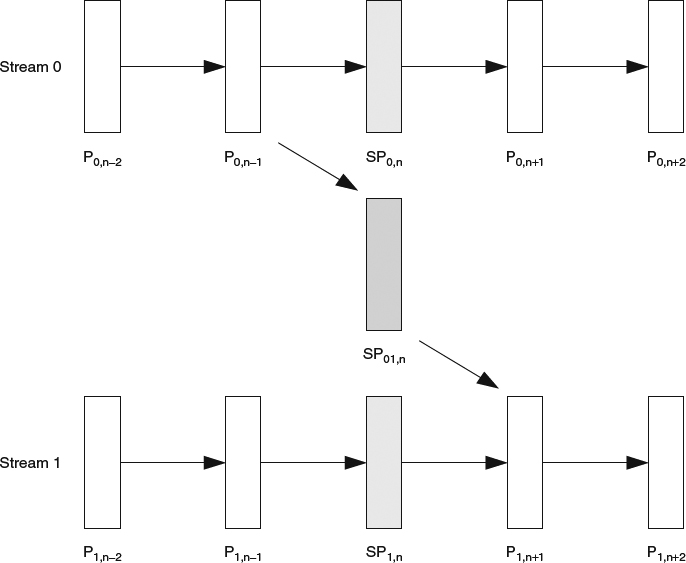
Figure 5.7 Bit stream switching using SP-frame.
We have seen the encoded bit stream in H.264 exhibiting strong decoding dependency owing to the advanced prediction and entropy coding, and so any bit error during the streaming process will cause error propagation until the next independent coding block. There are several coding tools developed in H.264 to address the issues for transmitting streams over error prone channels.
- Redundant slice: A slice can have another redundant representation in addition to its original version. In the error-free decoding process, the decoder will ignore the redundant slice. When a slice is found with errors, the decoder will find the associated redundant slice to replace this damaged slice. The penalty of the additional robustness brought by the redundant slices is the need of extra bandwidth to carry those redundant slices.
- Arbitrary slice order (ASO): H.264 defines a flexible syntax, first_mb_in_slice, to specify the position of the first macroblock in the current slice. Although the slice index always starts from 0 and grows monotonically, specifying first_mb_in_slice to a different value can physically change the slide order. For example, let's assume there are four slices in a video frame with resolution 1920 × 1088 and each slice has an equal number of MBs: (1920 × 1088)/(16 × 16)/4 = 2040 MBs. In other words, the aforementioned setting partitions a picture into four quarters. One can specify first_mb_in_slice in slice 0, 1, 2, and 3 as 2040, 6120, 0, and 4080. Slice 0, 1, 2, and 3 represent the second, fourth, first, and third quarters of the picture. With ASO, the codec is equipped with data interleaving ability to improve error resilience and to facilitate error concealment.
- Slide groups/flexible macroblock order (FSO): The macroblocks in a video frame can be grouped into several slices via a mapping table. In other words, the neighboring macroblocks can belong to different slices. Besides the traditional raster scan, six different map types of slice group are supported: interleaved/dispersed, explicit, foreground/background, box-out, and wipe. The slice group provides additional error resilience and a better base for error concealment. When a slice group is corrupted, the missing macroblocks in that slice group can be estimated from the other correctly received slice groups.
Recently, there has been a significant effort to standardize a new video codec, high efficiency video coding (HEVC) [6], which is based on the existing H.264 codec with lots of improved coding efficiency tools and software/hardware deployment consideration. The Joint Collaborative Team on Video Coding (JCT-VC) is a group of video coding experts from the ITU-T Study Group 16 (VCEG) and ISO/IEC JTC 1/SC 29/WG 11 (MPEG) to develop HEVC with a target of reducing by 50% the data rate needed for high quality video coding, as compared to the H.264/AVC standard. Although many coding tools are being added or improved, the overall decoder complexity is expected to be about twice that of H.264. There is no single encoding tool to boost the whole encoding efficiency, rather the encoding performance improvement is obtained by combining several coding tools.
- Coding hierarchy: The coding hierarchy of HEVC has major differences compared to H.264. A picture in HEVC consists of several nonoverlapped coding treeblocks, referred to as the largest coding unit (LCU). Each LCU can be further split into four sub-blocks via recursive quad-tree representation. If a sub-block has no further splitting, we call this sub-block a coding block, and a coding block can have size from 8 × 8 to 64 × 64. HEVC decouples the usage of blocks adopted in the prediction and transform processes. In other words, a block used in the transform process can cross the block boundary used in the prediction process. Prediction unit (PU) is defined in each CU and can have size from 4 × 4 to 64 × 64. Transform unit (TU) is defined in each CU and has block size from 4 × 4 to 32 × 32. The basic coding unit (CU) consists of PUs and TUs and associated coding data. In addition to the above coding hierarchy changes, to reduce the coding performance loss due to partitioning caused by slicing and to enable parallel processing, HEVC introduces the tile structure. Tiles are constructed by partitioning a picture horizontally and vertically into columns and rows. The partition boundary can be specified individually or uniformly spaced, and each tile is always rectangular with an integer number of LCUs.
- Intra-prediction: When a scene is captured by two different spatial resolution cameras, the object in the higher resolution image will include more pixels, and consequently there are more distinguished edge directions. As HEVC aims at supporting higher resolution images, the INTRA mode used in H.264 is not sufficient to cope with the larger image resolutions and bigger block size in CU. Advanced INTRA modes, including angular intra-prediction (33 different prediction directions), planar prediction, luma-based chroma prediction, mode dependent intra smoothing (MDIS), are added to improve the prediction performance.
- Inter-prediction: A similar problem is encountered in the inter-prediction for high spatial resolution content, as the small prediction unit used in H.264 cannot provide better compression performance. To achieve better prediction accuracy, a flexible partition size is introduced by including further partitioning of a CU to multiple PUs and asymmetric motion partition (AMP), which partitions a CU into unequal block size (for example, one PU with size 64 × 16 and one PU with size 64 × 48 inside one 64 × 64 CU). Other advanced coding tools, such as CU (PU) merging, advanced MV prediction (AMVP) via motion vector competition, 2D separable DCT-based interpolation filters (DCT-IF) for subpixel motion estimation/compensation, improved skip mode, and increased bit depth precision (14 bits) at the filter output, are included to enhance the compression performance.
- Transform: For higher resolution content, most image patterns in a block represent a small part of objects which can be described as homogeneous texture patterns with little variation. To take advantage of this, the residual quad-tree (RQT) is introduced by segmenting a CU into multiple transform blocks to fit into different size of homogeneous texture areas. Furthermore, the non-square quad-tree transform (NSQT) is included to tackle the scenario when a CU is split into non-square PUs (via AMP) or the scenario when the implicit TU splitting into four non-square TUs. The in-loop filtering used in HEVC is also refined by the three-step process: (1) deblocking, (2) sample adaptive offset (SAO), and (3) adaptive loop filtering (ALF).
- Entropy coding: In HEVC, the entropy coding component removes the CAVLC method and only adopts the CABAC method. The coefficients scanning (re-ordering) method adopted in HEVC CABAC is via a diagonal scan instead of the zigzag scan used in most video codec standards.
- Parallel processing: To enable parallel processing, the concept of wavefront processing is introduced. Wavefront parallel processing lets each LCU row run in its own decoding thread and each decoding thread proceeds to the next LCU immediately once its corresponding decoding dependency is resolved (such as the nearby top LCU being decoded).