8.1 Transmission-Induced Error

The transmission of video over a communication channel adds to the challenges associated with source compression, those arising from the errors that inevitably would be introduced in the channel. The presentation in Chapter 6 should have conveyed, among others, the message that while some channels are more benign, introducing errors less frequently than others, all channels do introduced errors. Therefore, when considering the quality of the communicated video from an end-to-end perspective, the experienced distortion will not only be due to the compression operation, but also due to channel errors. To differentiate these two types of distortions, we will be calling the former “source encoding distortion” or “source compression distortion”, and the latter “channel-induced distortion” or “transmission-induced distortion”.

Of course, channel errors will introduce a channel-induced distortion to the end-to-end video quality, but the magnitude of this distortion usually depends on several variables, such as the source encoding method used on the source, the error pattern introduced by the channel, the importance of the affected information from the human perception perspective, and so on. Indeed, practical video encoders frequently need to make use of and combine multiple techniques in order to achieve good compression performance. As a result, the bit stream at the output of a source encoder may be formed by different components, each having been generated by one of the data compression techniques. For example, in the bit stream at the output of a video encoder it is possible to find data related to the motion vectors obtained from using motion compensation, data related to a frame image or prediction error texture, which may result from differential encoding followed by entropy coding, data used to mark different parts in the bit stream, or headers carrying important metadata about the bit stream. The data being of different types, it is natural to see that channel errors will have different impacts on the source reconstruction quality for different parts of the source encoded bit stream. That is, while an error in one part of the bit stream may add a little distortion to the source reconstruction, an error of the same magnitude may have a devastating effect when affecting a different part of the bit stream.

The effects that the channel errors may have on the reconstruction quality of a source may differ depending on the importance of the parts affected or on the sensitivity of those parts to channel errors. One example of highly important parts within a source encoder bit stream are headers. The headers usually contain information that is indispensable for configuring the decoder. If this information is corrupted, then it simply may not be possible to decode a frame or a group of frames. In other cases, it may be that certain parts of the compressed video bit stream contain information that has been encoded with techniques that, while being more efficient, are more sensitive to channel errors. Sometimes this may happen due to the inherent structure of the encoded bit stream. For example, if using variable-length entropy coding, channel errors will have a more significant effect when affecting earlier bits. This is because all the succeeding bits will need to be discarded. In other cases, the higher sensitivity of a part of the compressed video bit stream may be due to using an encoding technique that is naturally more sensitive. This situation may occur, for example, when part of the information has been encoded using differential encoding, as is frequently the case with motion vectors. Because in differential encoding, one source encoded sample may depend on several previous samples, an error that is introduced for the reconstruction of a sample would affect several successive samples. We illustrate this point with the following simple example. Assume that a portion of a bit stream is encoding samples from a first order autoregressive Gaussian source x_n (n being the discrete time index) that behaves according to:

where w_n is the noise sequence, modeled as a discrete-time, zero-mean Gaussian random process with unit variance, and ρ controls the correlation between two successive samples. Since any given sample is correlated with the previous sample, it is natural to consider using differential encoding to compactly represent the samples x_n. A simplified form of the differential encoder and decoder is shown in Figure 8.1, for reference purposes. It can be seen how the encoder quantizes the error between the input sample and its value predicted from previous samples. In this case, the prediction can be implemented using a linear predictor that is just a one-tap prediction filter, with its only coefficient being a_o = ρ. That is, the linear predictor is an FIR filter with input–output difference equation, [1],

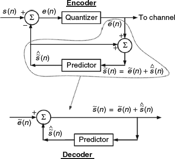
Figure 8.1 Block diagram for differential encoder and decoder.

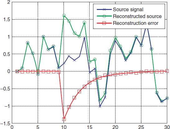
Figure 8.2 The effect of channel errors on a differentially encoded first order autoregressive Gaussian source. Channel errors are introduced only with the tenth transmitted error data.

It can be seen in Figure 8.1 that the transmitted data is in fact the quantized error between the input sample and its predicted value.

In this illustrative example, we now suppose that the channel introduces errors that only affect the tenth transmitted data. This data is subject to a binary symmetric channel with bit error rate of 10%. Figure 8.2 shows the impact of this error. As can be seen, before the tenth sample, when there have not been any channel errors, the reconstruction of the source follows the source quite faithfully. When the errors are introduced in the tenth transmitted data, the difference between the source and its reconstruction becomes large. This effect is, of course, as expected; but the higher sensitivity of differential encoding becomes evident as the error in the tenth transmitted data also affects the following samples through the prediction and differential methods used in the kernel of the decoder. The difference between the input source and its reconstruction decays slowly following the damped time constant given by the coefficient of the first order linear prediction filter. Of course, if it was possible to have errors with any of the transmitted data, not just the tenth one, the difference between the input source and its reconstruction would be significant at all times (see the example in Figure 8.3 with all transmissions going through a binary symmetric channel with bit error rate 0.1%).

The effect of channel errors on the reconstructed video also depends on the different importance of the compressed parts of the source or of the bits in the compressed video bit stream. The above-mentioned case of variable-length entropy coding is one example of the different importance for the bits in the bit stream. The case of compressing source information that is not equally important is crucial in video communication because it occurs often. Indeed, in video compression the unequal importance of the samples can be related to the different human subjective perception of sample distortion. We illustrate this case with an example using a simplified JPEG image compression scheme. The use of image compression here is only because it lends itself to an example that can be illustrated in a printed medium such as this book, but the observations are equally applicable to video compression. In this case we consider the source encoding and decoding of the image in Figure 8.4 using an eight-by-eight block discrete cosine transform (DCT) followed by quantization using the same quantization matrix and procedure followed in the JPEG image compression standard.

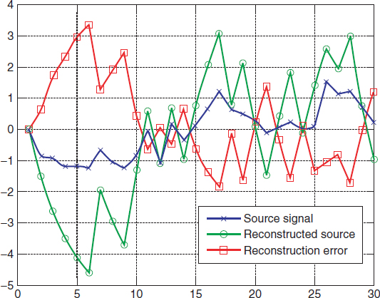
Figure 8.3 The effect of channel errors on a differentially encoded first order autoregressive Gaussian source when all the transmitted data is subject to a binary symmetric channel with bit error rate 0.1%.

The result of encoding and decoding without channel errors is shown in Figure 8.5, with the reconstructed image on the left and the corresponding pixel-by-pixel squared error on the right. For reference purposes, the measured peak signal-to-noise ratio (PSNR) in this case was 35.3 dB.

In terms of the block-based DCT technique used in JPEG and in this example, the DC coefficient is more important not only in terms of distortion associated with errors in this coefficient, but also in terms of human perception of the image quality. Figure 8.6 shows the same image after affecting the DC coefficients through a binary symmetric channel with bit error rate of 50% (this value of bit error rate is rather exaggerated in practical terms, but appropriate for this example). The figure shows the reconstructed image on the left and the corresponding pixel-by-pixel squared error on the right. In this case, the measured PSNR was 25.5 dB, a value that is also evident from the clearly distorted result in the figure.

Figure 8.4 Original image to be encoded and decoded using a simplified JPEG technique.

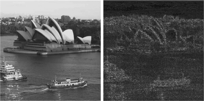
Figure 8.5 The recovered image from Figure 8.4, after encoding and decoding. On the left, the reconstructed image and on the right the corresponding squared error.

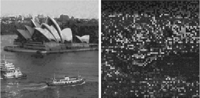
Figure 8.6 The recovered image from Figure 8.4, after encoding and decoding when the DC coefficients of the block DCT transforms are transmitted through a binary symmetric channel with bit error rate 50%. On the left, the reconstructed image and on the right the corresponding squared error.

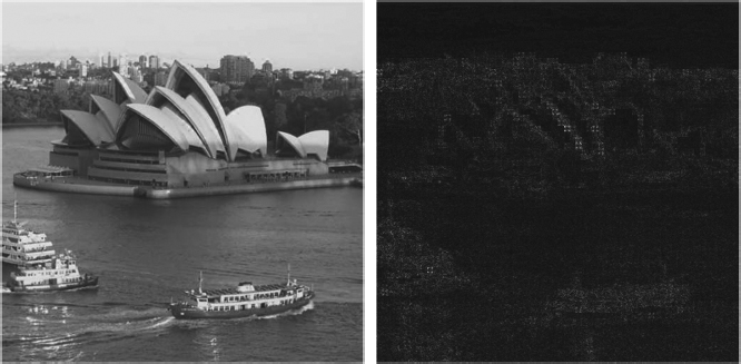
Figure 8.7 The recovered image from Figure 8.4, after encoding and decoding the coefficients with coordinates (1,1) of the block DCT transforms, are transmitted through a binary symmetric channel with bit error rate 50%. On the left, the reconstructed image and on the right the corresponding squared error.

The DC coefficient is the most important one, and the rest of the coefficients are not as important. Figure 8.7 shows the same image, after affecting the coefficients with coordinates (1,1) by the same binary symmetric channel with bit error rate of 50% as was used for the DC coefficients. The figure shows the reconstructed image on the left and the corresponding pixel-by-pixel squared error on the right. In this case, the measured PSNR was 34.7 dB, roughly 0.5 dB less than the case with no channel errors. In this case, the errors are so difficult to perceive that the figure that shows the pixel-by-pixel squared error becomes indispensable. In this figure, it can be seen that the biggest distortion is introduced in areas of the original image with some edges in the texture, for example the edges of the seashell-shaped roof of Sydney's opera house.

In multi-view video, there are cases where in the output bit stream from the video compressor it is possible to recognize two parts: one containing color and texture information, and another containing video depth information. This organization is useful in certain applications where the color information can be used to provide backwards compatibility with legacy 2D video systems. It was observed in [2] that the channel errors have a more negative effect in terms of distortion over the color information and less of a negative effect on the video depth information.

In general, the modeling of channel-induced distortion for multi-view video sequences is a complex task. This is because the encoding–decoding process depends on the application of a number of techniques but, more importantly, because the use of differential encoding in both the time domain and between different views creates error propagation effects with complex interrelations in the time and in the inter-view dimensions. The modeling of channel-induced distortion for multi-view video was studied in [3]. In this case, the source encoder exploits the correlation in time and between views. Specifically, denoting by M(s, t) the frame from view s at time t, most of the views are assumed to encode a frame using differential encoding from the previous frame in time, M(s, t − 1), and in the view domain, M(s − 1, t). The only exception to this encoding structure is a view, identified as “view 0”, which starts a group of pictures (GoPs) with an intra-predicted frame, encoded independently of any other frame, and follows with frames that are encoded using differential encoding only in the time domain.

Having introduced the encoding model and basic notation, it is possible to illustrate the complexity involved with the modeling of channel-induced distortion with multi-view video. Suppose that a frame M(s, t) is affected by errors during transmission. For this frame it will be necessary to estimate the effects of the errors. Yet, the errors will propagate to frames M(s + 1, t), M(s + 2, t), …, M(s + S, t), assuming that there are S views, and to frames M(s, t + 1), M (s, t + 2),…, M(s, t + T), assuming that there are T frames in a GoPs. The propagation of the errors will depend on such factors as the nature of the prediction done during differential encoding, how errors are concealed, and so on. Furthermore, for as much as the previous case assumes the presence of errors in a single frame M(s, t), in practice these errors will occur in multiple frames, creating a complex pattern of interweaved error propagation effects.

To model channel-induced distortion, the work in [3] starts by assuming that the presence of an error in a frame that leads to the loss of a packet results, in turn, in the loss of the complete frame. Also, analytical studies for very simple source and channel coding schemes and video communication simulations all point toward an end-to-end distortion model where the frame source encoding distortion, D_s (s, t), and the frame channel-induced distortion, D_c (s, t), are uncorrelated. Therefore, the end-to-end distortion can be written as:

Modeling the channel-induced distortion implies focusing only on the term D_c(s, t).

Let P be the probability of losing a packet and, consequently, also the probability of losing a frame. For a given frame M(s, t), the mean channel-induced distortion follows from the channel-induced distortion when frame M(s, t) is lost, D_L(s, t), and the channel-induced distortion when frame M(s, t) is not lost but is being affected by error propagation from a previous-time or previous-view frame, D_NL(s, t):

Inter-predicted frames usually switch between macroblocks encoded inter- or intra-prediction. The decision on whether to use one or the other mode is based on an estimation of the resulting distortion. When the frame M(s, t) was not lost, the channel-induced distortion is for the most part due to the propagation of errors that affected a previous frame. These errors may also affect the portion of the frame that is encoded using intra-prediction, as there is a correlation through the decision on whether or not to use intra-prediction, but it has been observed that this effect is negligible. As a consequence, if the average proportion of macroblocks encoded using intra-prediction is Q, the channel-induced distortion in this case can be written as:

where V is the percentage of proportion of macroblocks using differential encoding in the time domain, and λ_b and λ_a are values related with the error-introduced distortion rate of decay while an error propagates when using differential encoding on the view and the time domain, respectively. The two values λ_b and λ_a are intended to capture the gradual decrease in the value of the propagating distortion due to the filtering operation embedded within the prediction in differential encoding, as illustrated with the simple example in Figure 8.2.

When a packet is lost, it is assumed in [3] that this also creates the loss of a frame. Consequently, the study of the channel-induced distortion when a frame M(s, t) is lost also needs to consider how to replace the lost information. This technique, called “error concealment”, will be studied in more detail later in this chapter. In the case of the study in [3], the concealment of lost information is implemented in a very simple way, by replacing the lost frame with a copy of the frame in the previous view or time. If the proportion of frames replaced using a copy of the previous frame in time is U, the channel induced distortion when a frame is lost can be written as:

where D_LT(s, t) is the average distortion when replacing a lost frame with the previous frame in time and D_LV(s, t) is the average distortion when replacing a lost frame with the frame in the previous view.

The model for D_LT (s, t) is essentially the same as when considering a single-view video and can be written as:

This expression splits the distortion D_LT(s, t) into two terms. The first term, D_TEC (s, t), is the distortion due to replacing a lost frame with the previous temporal frame. The second term, μ_bD_c(s, t − 1), characterizes the distortion due to transmission errors, where μ_b is the value modeling the gradual decay in error-introduced distortion when using differential encoding. The value of μ_b may differ from λ_b because in principle the predictors may be operating with different data.

With similar arguments, the distortion D_LV (s, t) can be written as:

where it is possible to recognize the same two terms, with analogous variables and functions, as in the expression for D_LT(s, t).

Since D_c (s, t) = (1 − P)D_NL(s, t) + P D_L(s, t), it is now possible to combine all the different components of the channel-induced distortion shown above to get:

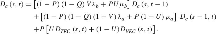
As can be seen, the channel-induced distortion depends on the distortion performance delivered by the error concealment scheme being used, and the distortion from previous temporal and view frames. The degree to which the channel-induced distortion from previous frames decreases over time depends on the values [(1 − P)(1 − Q)Vλ_b + PUμ_b] and [(1 − P)(1 − Q)(1 − V)λ_a + P(1 − U)μ_a] for the time domain and previous view domain. These values depend on the statistics of the video sequence and characteristics of the video encoder.

As a summary of this section, we note that errors introduced during transmission of compressed video will have an effect on end-to-end distortion that will be combined with the distortion already introduced during the video compression stage. The magnitude of the channel error effect will depend on several factors related to the communication process itself. In the rest of this chapter we will be focusing on channel-induced errors and their effect on end-to-end distortion. We will discuss techniques to reduce the sensitivity to errors, to recover from them, and to efficiently protect against them.