7.2 QoE Measurement

The 3D artifacts produced from the current 3D technology pipeline have been introduced in the previous section. Ultimately, a human observer is the final quality determiner and it is important to conduct 3D video quality assessment to measure and ensure the quality of experience (QoE). Therefore, it is of interest to evaluate the perception of 3D videos in the process of acquisition, communication, and processing. Quality assessment (QA) is the term used for techniques that attempt to quantify the quality of a 3D signal as seen by a human observer. Generally, quality assessment plays a key role in 3D video processing because it can be used to:

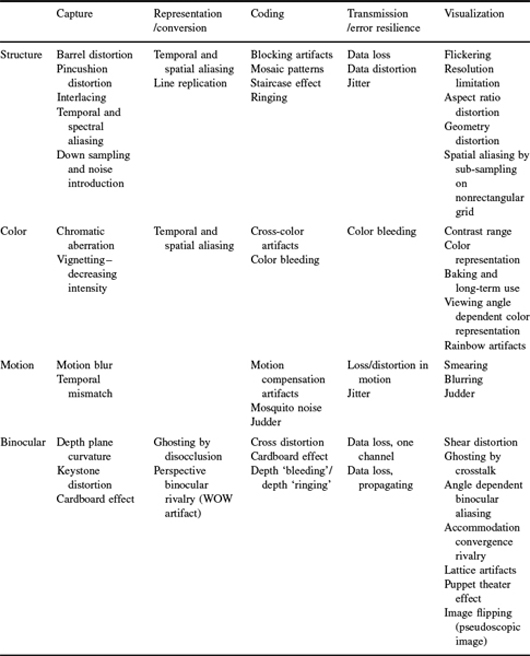
Table 7.1 Summary of the artifacts for the 3D artifacts [2]. In addition to the stereoscopic artifact, the autostereoscopic display may have unique artifacts, crosstalk, showing up in display [19]. Crosstalk is caused by imperfect separation of the left and right view images and is perceived as ghosting artifacts. The magnitude of crosstalk is affected by two factors: position of the observer and quality of the optical filter. The extreme of crosstalk is the pseudoscopic (reversed stereo) image when the left eye sees the image representing the right view and the right eye sees the image representing the left view

• monitor delivered quality: 3D perceptual degradation is possibly introduced during the process of video capturing, transmitting, and synthesizing resource. Monitoring the delivered quality gives the service provider the ability to adjust allocation strategies to meet the requirements of QoE,
• evaluate performance: a quality assessment provides a means to evaluate the perceptual performance of 3D capturing, processing, transmitting, and synthesizing systems,
• optimize 3D video processing procedure: a system can be designed to either satisfy a specific maximal perceptual distortion with minimal resource allocation or minimize the possible perceptual distortion with a proper perceptual quality assessment metric.

Image and video quality assessments have been research topics for the past few decades. 3D videos extend the concept of 2D videos by adding the extra depth for the stereoscopic perception of the 3D world. Thus, the quality assessment of 3D videos should be closely related to the concepts of 2D videos and image quality assessment methods. Thus, this section will first review several important aspects and techniques in image and video quality assessment. Then, several current available 3D video quality assessments will be discussed.

7.2.1 Subjective Evaluations

Since humans are the ultimate judge of the 3D contents delivered, subjective studies are generally used for 3D system development in choosing the algorithms for the system pipeline, optimizing the system parameters or developing objective quality assessments. In this section, a short review is given, and then two commonly used methods are introduced.

Generally the subjective studies can be categorized as:

1. Psychoperceptual approaches

   In 1974, ITU-R BT.500 [20] was published by the International Telecommunication Union (ITU) as the recommendation for conducting psychoperceptual studies focusing on television pictures. The recommendation was adjusted for evaluating stereoscopic content to become ITU-R BT.1438 [21]. These ITU recommendations focus on measuring subjective and human perceptual quality. The evaluation is either based on pair comparisons of stimuli to judge the perceived differences, or on single-stimulus methods of rating the stimuli independently. Psychoperceptual approaches generally create preference orders of the stimuli for understanding the impact of parameters on human perceptual video quality.

2. User-centered approaches

   The user-centered approaches expand subjective quality evaluation toward the human behavioral level. Quality of perception (QoP) [22] can link the viewers' overall acceptance of the presented content and their ability to understand the information contained in the content. However, QoP does not discover the quality acceptance threshold. Studies [23, 24] discover the acceptance threshold based on Fechner's method of limits and use a bi-dimensional measure to combine retrospective overall quality acceptance and satisfaction. The results of the study reveal the identification of the acceptance threshold and a preference analysis of the stimuli. Generally, the studies of evaluation are conducted in a controlled environment but quality evaluation in the context of use has become more important for 3D systems. Therefore, research [25, 26] has tried to close the gap using so-called quasi-experimental settings which represent a new concept to conduct experiments without full control over potential causal events.

3. Descriptive quality approaches

   These methods focus on discovering quality factors and/or their relationship to quality preferences. As demonstrated in [27], the result of several predefined variables should not be viewed as subjective quality measurements, and the study should be open in order to understand underlying quality factors. The approaches used are different from the first two categories. Interviews [27] and other studies such as the sensory profiling approaches [28] are used to discover quality factors that the users experience. Radum et al. [29] adapted the concept to study the perception of still images and Strohmeier et al. [30] applied the free choice profiling approach [31] to study the perception of audiovisual and stereoscopic videos.

These three different categories of subjective quality methods have different research focuses. Psychoperceptual studies [20, 21, 32] are highly controlled and they focus on the quality preferences. User-centered studies [22–24] expand the evaluation to the actual use of the system. Descriptive studies [27–29] try to discover the factors that affect viewers' perceptual quality. Jumisko et al. [23] provided an overview of existing psychoperceptual, user-center, and descriptive evaluation methods and their applications in stereoscopic video quality studies. However, in order to do a proper quality evaluation which can study the quality as a whole according to users, the system, and context of use, a 3D quality research must create a framework considering all the mentioned aspects in three categories.

7.2.1.1 Open Profiling Quality (OPQ)

OPQ [33–35] is a subjective method for 3D quality assessment and is a method which can evaluate the quality preferences and elicit the idiosyncratic quality factors. OPQ adapts free choice profiling to do quantitative psychoperceptual evaluation. The goals of the method are:

1. to find out how good the perception quality is,
2. to discover the perception factors,
3. to build a relation between user preferences and quality factors,
4. to provide researchers a simple and naive test methodology.

Researchers can use OPQ to study the parameters and attributes for quality assessments. In other words, it is up to researchers to find out what viewers perceive as quality factors.

1. Procedure

   Strohmeier et al. [34, 35] described the procedure of OPQ in detail. Based on the recommendations [20], a psychoperceptual evaluation is conducted for participants to evaluate the acceptance and satisfaction with the overall quality. Free choice profiling [31] is adapted to conduct a sensory profiling evaluation. This profiling allows participants to use their own vocabulary for the evaluation of overall quality. As shown in Figure 7.6, the main steps are as follows:

   (a) An introduction of quality elicitation is given.

   (b) Participants discover the factors based on their own vocabularies which are preferably adjectives.

   (c) Participants refine their final vocabularies to identify the factors that are unique and can be precisely identified by the researchers.

   (d) After refinement, the participants score these factors as they are presented with the stimuli one after another for stimulus evaluation.

   Figure 7.7 shows the outline of traditional psychoperceptual quality evaluation. The main difference is that the OPQ splits the second step of the traditional psychoperceptual quality evaluation into two steps: attribute finding and attribute refinement.

2. Analysis

   After applying OPQ, a quantitative data set and sensory data set are generated. Analysis of variance is applied to the quantitative data for a preference ranking. Then, generalized procrustes analysis (GPA) is applied to the sensory data to create a low-dimensional perceptual model which shows the principal components separating the test items and correlating with idiosyncratic factors. With further analysis of the model, deeper insight can be obtained to explain the quality preferences shown in the quantitative data. Finally, external preference mapping [36] is applied to link the preference and the perception model, that is, quality factors.

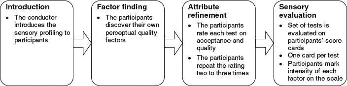
Figure 7.6 The flow diagram of the main steps executed in the process of OPQ.

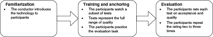
Figure 7.7 The flow diagram of the general steps conducted in psychoperceptual quality evaluation.

7.2.1.2 User-centered Quality of Experience

Because we are evaluating the produced quality of 3D dynamic and heterogeneous contexts in consumer services, conventional quality evaluation methods are questionable. In order to conduct evaluation, a quasi-experimental evaluation and novel tools for the evaluation procedure are required for conducting research in quality evaluation outside controlled laboratory conditions. User-centered quality of experience [37, 38] is for quality evaluation in the natural circumstances. Generally, the context used in the study can be described in terms of:

1. macro, that is a high-level description of the contexts, for example, describing the context capturing a certain type of scenes under certain conditions,
2. micro, that is a situational description, for example, describing the context in a second-by-second manner.

The quality evaluation in the context of use requires a hybrid data-collection and analysis procedure. This method is composed of the following three phases:

1. Planning Phase

   Fundamentally, this phase analyzes macro information of the contexts and their characteristics. The following describes the two main steps:

   (a) Select the contexts based on the research requirements: Because the length of experiments must be reasonable, only a certain number of contexts can be presented. The chosen contexts should be the most common and diverse to gather the heterogeneity of extreme circumstances. The content used in stereoscopic quality assessments can be categorized as:

   i. physically, which mainly focuses on the place where the 3D devices are watched such as at home or in a hall [39–44],

   ii. temporally, which mainly focuses on the length of the 3D contents [39, 40, 44, 45] and the time when watching events happen [43],

   iii. socially, which mainly focuses on the social interactions which vary from solo-viewing [40, 42] to co-viewing [39–40, 42],

   iv. task-orientedly, technically, and informatively, which mainly focuses on the degree of attention needed to achieve the viewer's goal such as high concentration [40] and low concentration [39, 42, 45].

   (b) Analyze the characteristics of chosen contexts: A semantic description and more detailed and systematic analysis must be given to the chosen context in order to understand what the right conditions are for the experiment to take place. For example, usability study of mobile 3DTV conducted in [37] uses CoU-MHCI form [46] to characterize the chosen contexts and to list the potential threads to causal interference as discussed in [25]. Instructions to the participants and operators are written in order to avoid the mono-operation bias. A pilot test can also help the researchers to check the relevance of selected situations and testing equipment and algorithms. Finally, back-up plans are needed to deal with changes that happen during the experiments.

2. Data-collection Phase

   The data-collection phase contains the following six parts:

   (a) Quality evaluation task: A simple evaluation method is used to rate the preference of overall quality after applying each stimulus using a simple evaluation task, because it is desirable to know whether the presented quality reaches an acceptable threshold for the usage of the consumer technologies [23]. Generally, the main challenge in this task is to maximize the range of contexts and minimize the evaluation obstruction.

   (b) Structured observation by the conductor: During the evaluation procedure, the conductor instructs the participants and observes and records the situations and conditions of the evaluation procedures with the aid of a semi-structured observation form such as [47, 37].

   (c) Work-load assessment of quality evaluation: After each evaluation task, the overall experiences of the evaluation in terms of mental demand, physical demand, time pressure, effort, frustration, and performance are investigated with a questionnaire such as NASA-TLX [48].

   (d) Interview about quality of used contexts: An interview about experiences and impressions of quality in the context is conducted by the conductor during the time between contexts. The interview should be collected naturally and casually to get the first impressions of quality in the context.

   (e) Interview about experiences of quality: Following contextual evaluations, the conductors conduct broader semi-structured interview about the experiences of the quality context and quality. The importance of the interview is mainly for discovering the experiences of perceived quality and requirements for good perception.

   (f) Situational data-collection audio-video recording of the experiment: The entire experimental process is recorded with video cameras and microphones [49].

   Parts (a) to (e) describe the macro-level data-collection tools in a context while part (f) targets the micro-level analysis of context.

3. Analysis Phase

   First, the collected data is analyzed separately and then the analyzed results are integrated as:

   (a) characteristics of center of use (CoU): This focuses on identifying central values of the actual characteristics of contexts of use to count participants' CoU.

   (b) contextual influences on quality: This focuses on statistically analyzing the influence of used context on quality requirements and workload.

   (c) linkage between the interview: This focuses on linking the contextual quality experience with the interview data about experience of contexts and situational audio-video recordings based on data-driven frameworks.

7.2.2 2D Image and Video QoE Measurement

Since the content is ultimately consumed by humans and the quality of these video contents affects the perception of viewers, the subjective assessment of the image and video quality is needed and preferred. However, the subjective methods are generally expensive and time-consuming and require good knowledge and deep efforts to collect meaningful ratings from a group of subjects. Furthermore, the subjective assessment methods cannot be applied to all images and videos of interest. Therefore, an automatic algorithm, which is objective and not affected by mood, expectation, past experience, or other factors inherent in human subjects, is required to better achieve the goal of evaluation described previously. The goal of an objective perceptual metric uses a number to represent the probability that a human eye can detect the distortions of an image or video or the difference between two images or videos. Alternatively, a map can be used to represent the probability of a distortion detected on that pixel of an image or video or the difference between two images or videos. Wang et al. [50] and Winkler et al. [51] categorized objective metrics according to the amount of information required from the reference image or video to evaluate the degree of distortions:

• Full-reference (FR) metrics require the entire original image or video as the reference for quality evaluation. The requirement is generally fulfilled in compression, restoration, enhancement, and reproduction applications in the server side. The goal of FR algorithms is to evaluate the fidelity of the test or distorted video compared to the reference video. This category is still the main focus and thus most algorithms discussed in this section belong to this category.
• Reduced-reference (RR) metrics extract a fixed number of features from the reference image or video and use them as reference to evaluate the quality of the image or video. Generally, the algorithm is used to evaluate the efficiency of streaming and broadcasting applications because the full reference image or video is not available in the client side. The representative researches are [50, 52–57].
• No-reference (NR) metrics or blind algorithms attempt to evaluate the quality of an image or video without any other reference information. Generally, it is designed to detect the distortions generated by specific applications such as blocking (typically generated in the process of discrete cosine transform), ringing, and blurring. Several NR algorithms have been proposed to evaluate the contrast, sharpness, color saturation, and presence of noise in an image or video. However, NR-based methods still remain difficult problems to combine all these affecting factors into a meaningful metric [58].

Furthermore, the quality assessments can also be categorized according to the types of operation conducted.

1. Pixel-based metrics

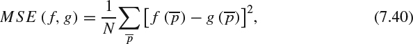
   These metrics are probably the earliest and most commonly used quality metrics because of their simplicity. The representatives are the mean square error (MSE) and the peak signal-to-noise ratio (PSNR) difference metrics. and are the values of an image pixel at location for the image f and g, where . The MSE can be computed as:

   

   where N is the total number of pixel in the images. PSNR can be computed as:

   

   where E is the maximum value that an image can have in this representation. For example, E = 255 for 8-bit gray-scale image. Both PSNR and MSE can be directly applied to a 2D video by accumulating the error in all pixels in all frames, and a 3D video by accumulating errors in all pixels of both views in all frames. However, the most arguable issue of using MSE and PSNR is that they do not directly reflect the perception of human eyes. Thus, the number computed cannot truly reflect the real perceived distortions of images or videos.

2. Human vision system based metrics

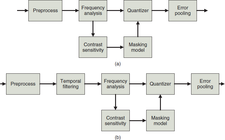
   Psychophysics has modeled the human vision system as a sequence of processing stages which are described by a set of mathematical equations. Human vision system (HVS) based metrics evaluate the quality of an image or video based on these sets of mathematical models. These metrics first compute the threshold of distortion visibility and then apply the thresholds to normalize the error between the test and reference content to get a perceptual metric. In order to compute the threshold of distortion visibility, different aspects in the visual processing procedure must be considered, such as luminance response, contrast, spatial frequencies, and orientations; HVS based metrics then attempt to model these aspects into different HVS processing stages that induce different observed visibility thresholds. Generally, an HVS based image quality assessment system consists of a set of blocks shown in Figure 7.8a. To address the additional time domain information brought by a video, there is an extra block for temporal processing in the HVS based video quality assessment, as illustrated in Figure 7.8b. The following gives a short description of each block.

   

   Figure 7.8 (a) HVS-based image quality assessment blocks. (b) HVS-based video quality assessment blocks.

   • Preprocessing: The preprocessing step generally comprises two substeps: calibration and registration. The calibration process is used to remove the color and viewing bias by applying a mapping algorithm from values to units of visual frequencies or cycles per degree of visual angle. It was proposed in [59–61] that the input parameters include the viewing distance, physical pixel distance, fixation depth, eccentricity of the images in the observer visual field, and display related parameters. Registration establishes the point-to-point correspondence between the test and reference images or videos. Without this step, misaligned pairs will introduce shifting in the pixel domain or in the selected coefficient values and degrade the system performance.
   • Frequency analysis: The HVS responds differently to different spatial frequencies and orientations and therefore this stage fundamentally simulates HVS spatial component response: neurons in the brain respond selectively to spatial signal components with particular frequencies and orientations by using frequency trans-formation to transform an image or video into components having different color channels with different spatial frequencies and orientations.
   • Contrast sensitivity: The contrast sensitivity function (CSF) characterizes the frequency response of HVS and is also called the modulation transfer function (MTF). The action of CSF can be simulated by the response of a set of bandpass filters. Since the spatial frequencies are measured in the units of cycles per degree of visual angle, the viewing distance affects the visibility of details at a particular frequency. Quality metrics generally define a minimum viewing distance where distortion is maximally detectable and evaluate the distortion metric at that point. The contrast sensitivity denotes the amount of change in a flat mid-gray image in each frequency that can be detected. Sometimes it is also called just noticeable difference (JND).
   • Luminance masking: An eye's perception of lightness is not a linear function of the luminance. Sometimes this phenomenon is called light adaptation or luminance masking because the luminance of the original image signal masks the distortions of the distorted images. The effect is generally computed along with other masking effect in the masking block [62].
   • Contrast masking: Psychophysical experiments generally use an assumption of simple contents. However, natural scenes contain a wide range of frequencies and different scale contents. In addition, the HVS is a nonlinear system and the CSF cannot completely describe the behavior of the response for any arbitrary input. Therefore Robson et al. [63] and Leggel et al. [64] proposed that contrast masking refers to the reduction in detection of an image component under the presence of other image components with a similar spatial location and frequency content.
   • Error pooling: The final process is to combine all errors from the output of different psychophysical models into a single number for each pixel of the image or video or a single number for the entire image or video.
   • Temporal filtering: Videos contain a sequence of images and have different effects on the detection of image components. Generally, a spatiotemporal filter is separable along the spatial and temporal dimensions. Temporal filters use linear low-pass and bandpass filters to model two early visual coretex processing mechanisms. The temporal filtering utilizes a Gabor filter. Furthermore, the CSF is measured as a nonseparable function of spatial and temporal frequencies using psychophysical experiments.

   In the following we will summarize several quality assessment models including the visible differences predictor (VDP), the Sarnoff JND vision model, the Teo and Heeger model, visual signal-to-noise ratio (VSNR), moving pictures quality metric (MPQM), perceptual distortion metric (PDM), peak signal-noise-ratio-based on human visual system metric (PSNR-HVS), and modified peak signal-noise-ratio based human visual system (PSNR-HVS-M).

   (a) Visible difference predictor (VDP): The VDP is developed for high quality image systems [59]. Frequency analysis is done with a variation of the cortex transformation. Contrast sensitivity uses the CSF which models luminance masking or amplitude nonlinearities using a point-by-point nonlinearity, and contrast masking is done with two alternative methods: local contrast and global contrast. To account for the complex content in a natural image, an experimental result of masking is used to help the masking. Error pooling is done with a map which represents the computational result of the probability of discriminating the difference in each pixel between the reference and testing image.

   (b) Sarnoff JND vision model [60]: The algorithm applies preprocessing steps to consider the viewing distance, fixation depth, and eccentricity of the observers' visual field. Burt et al. [65] proposed to use Laplacian pyramid for frequency analysis. Freeman et al. [66] used two Hilbert transform pairs for computing the orientation of the signal. The contrast sensitivity is normalized by the CSF for that position and pyramid level. A transducer or a contrast gain control model is used to model the adaptation of response to the ambient contrast of the stimulus. A Minkowski error between the responses of the test and reference images is computed and converted to the distance measurement using a psychometric function. The measurement represents a probability value for the discrimination of the test and reference image.

   (c) Teo and Heeger model [67]: Frequency analysis is done with the steerable pyramid transform in [68] which decomposes the image into several spatial frequency and orientation bands. In addition, it combines the contrast sensitivity and contrast masking effects into a normalization model to explain baseline contrast sensitivity, contrast masking, and orientation masking that occur when the orientations of the target and the mask are different. The error pooling uses the Minkowski error which is similar to Sarnoff JND.

   (d) Visual signal-to-noise ratio (VSNR) [69]: VSNR is different from those methods discussed previously in three aspects:

   i. VSNR computational models are derived from the results of psychophysical experiments on detecting visual distortions in natural images.

   ii. VSNR is designed to measure the perceived contrast of supra-threshold distortion not just a threshold of visibility.

   iii. VSNR is also designed to capture a mid-level property of the HVS known as global precedence when comparing to capturing low-level processes in the visual system.

   Basically, the preprocessing considers the effect of viewing conditions and display characteristics. Frequency analysis uses the decomposition of an M-level discrete wavelet transform using the 9/7 bi-orthogonal filters. The average contrast signal-to-noise ratios (CSNR) is computed as a threshold to detect distortions in the transformation. VSNR applies the contrast constancy using RMS to scale the error for using a measurement of the perceived distortion, d_pc. Contrast constancy is that the perceived change in supra-threshold range generally depends much less on spatial frequency than those predicted by the CSF. The HVS has the preference of integrating edges in a coarse-to-fine scale fashion. A global contrast precedence model is used to compute the detected contrast distortion magnitude, d_gp. Error pooling is the linear combination of d_pc and d_gp.

   (e) Moving pictures quality metric (MPQM) [70]: Frequency analysis uses a Gabor filter bank. The temporal filtering mechanism uses a combination of a bandpass filter and a low-pass filter. Furthermore, the contrast sensitivity function uses a non-separable function of spatial and temporal frequencies built from psychophysical experiments.

   (f) Perceptual distortion metric (PDM) [71]: Frequency analysis uses the steerable pyramid, and temporal filtering uses two infinite impulse response (IIR) filters to model the low-pass and bandpass mechanisms [72].

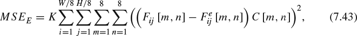
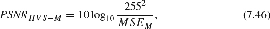
   (g) Peak signal-noise-ratio-based on human visual system metric (PSNR-HVS) [73]: PSNR-HVS computes PSNR with consideration of the peculiarities of the human visual system (HVS). Past studies show that the HVS is more sensitive to low frequency distortions rather than to high frequency on. In addition, the HVS is also sensitive to contrast and noise. DCT can provide the de-correlation and the correlation information to the visual perception and, therefore, the PSNR-HVS can be computed as:

   

   where MSE_E is computed when considering the HVS characteristics in the following manners:

   

   where W and H are the width and height of the image respectively, K = 1/WH is a normalization constant, F_ij are 8 × 8 DCT coefficients of the 8 × 8 image block whose left upper corner locates at [8i, 8j], F_ij [m, n] is the coefficient whose location is at m and n inside the block of F_ij, is the DCT coefficients of the corresponding block in the reference image, and C is the matrix of the correcting constants [73].

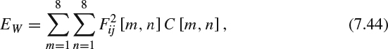
   (h) Modified peak signal-noise-ratio-based on human visual system metric (PSNR-HVS): Ponomarenko et al. [74] extend PSNR-HVS to take the CSF into account and use 8 × 8 DCT basis functions to estimate between-coefficient contrast masking effects. The model can compute the maximal distortion of each DCT coefficient which is not visible due to the between-coefficient masking. The masking degree at each coefficient F_ij [m, n] depends on its power and the human eye sensitivity to the DCT basis function based on the means of the CSF:

   

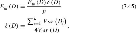
   where F_ij [m, n] is the DCT coefficient which is the same as the one used in PSNR-HVS, C [m, n] is a correcting constant calculated using the CSF and computed from normalizing quantization table used in JPEG [75]. The algorithm assumes that two sets of DCT coefficients, F_ij and G_ij, are visually undistinguished if E_W(F_ij − G_ij) < max(E_W(F_ij)/16, E_W(G_ij)/16), where E_W(F_ij)/16 models a masking effect. Edge presence can reduce the masking effect in the analyzed image block D. Divide the 8 × 8 image D into four 4 × 4 sub-blocks D₁, D₂, D₃, and D₄. PSNR-HVS-M proposes that the strength of this masking effect is proportional to the local variance Var(D):

   

   where the normalizing factor p = 16 has been selected experimentally, Var(D) is the variance of all the DCT coefficients in the 8 × 8 block D and Var (D_i) is the variance of all the DCT coefficients in the 4 × 4 sub-block D_i. And the error metrics can be computed as:

   

   where MSE_M is computed as

   

3. Structure based or feature based metrics

   Since the HVS is strongly specialized in learning about scenes through extracting structural information, it can be expected that the perceived image quality can be well approximated by measuring structural distortions between images.

   The algorithms extract features computed from the reference and test images or videos and then compare the extracted features for measuring the quality of the test video. Feature based approaches form the bases of several no-reference quality assessments which are discussed in [55]. Depending on how structural information and structural distortions are defined, there are several different quality assessments:

   (a) The structural similarity (SSIM) index: Wang et al. [76] observed that the luminance of the surfaces on an object is the product of the illumination and the reflectance but is independent of the structures of the object. As a result, during the analysis of perception, it is better to separate the influence of illumination from the structural information of the object. Intuitively, the illumination change should have a main impact on the variation of the local luminance and contrast but such variation should not have a strong effect on the structural perception of the image. Therefore, SSIM is set up to compute the image quality based on the structural information in the following steps:

   i. The mean intensity of each image is computed as the luminance.

   ii. A luminance comparison function is then defined with the mean intensity, and the standard deviation of each patch is computed to define the contrast of that patch.

   iii. The value in each pixel is normalized with its own standard deviation for structural comparison.

   As a result, the SSIM index is computed as a combination of the three comparison functions: luminance, contrast, and structure. The structure term is the most important term in SSIM and should not be affected by the luminance and contrast change. Error pooling is done with a weighted linear combination of all SSIM indices.

   (b) The perceptual evaluation of video quality (PEVQ) [77–80]: PEVQ is developed based on the perceptual video quality measure (PVQM) [78]. From the reference and test videos for perceptual analysis, these algorithms compute three indicators: an edginess indicator, a temporal indicator, and a chrominance indicator. The edginess indicator gives the information of the structural differences between the reference and test videos and is to compare the edge structure between the reference and test videos where the edge structure is approximated using the local gradients of the luminance of the frames in the videos. The temporal indicator defines the amount of movement or change in the video sequence and is computed as a normalized cross-correlation between adjacent frames of the video. The chrominance indicator provides the perceived difference in chrominance or color between the reference and test videos and is computed similarly to the contrast masking procedure. Finally, these indicators are combined into a mapping for measuring the visual quality of the test video.

   (c) The video quality metric (VQM) [81]: The VQM contains the following processing steps:

   i. Preprocessing steps calibrate the reference and test sequences, align them spatially and temporally, extract valid regions from the videos, and obtain the gain and offset correction [81, 82].

   ii. Features are extracted from spatiotemporal subregions of the reference and test videos. The VQM computes seven parameters from the feature streams. Four of the seven parameters are based on features extracted from the spatial gradient of the luminance in the videos. Another two components are computed from the chrominance components. The number of spatial and temporal details affects the perceptibility of temporal and spatial impairments in a video. The final parameter is computed as the product of a contrast feature that measures the number of spatial details and a temporal feature for temporal details.

   iii. A spatiotemporally local quality parameter is computed using one of the following three comparison functions that emulate the perception of impairments: a Euclidean distance, a ratio comparison and a log comparison. The three comparison functions in VQM have been developed to account for visual masking properties of videos.

   iv. Error pooling computes a single quality score using spatial pooling and temporal pooling functions. The spatial pooling functions are defined with the mean, standard deviation, and worst-case quantile defined in statistics [83]. The temporal pooling functions are defined with the mean, standard deviation, worst-case quantile and best-case quantile of the time history of the videos.

4. Information theoretic approaches

   Information theoretic quality assessments view the quality as an information fidelity problem rather than a signal fidelity problem. An image or video is sent to the receiver through a channel with limited communication ability and therefore distortions are introduced into the receiving information. The input to the communication channel is the reference image or video, and the output of the receiving channel is the test image or video and visual quality is measured as the amount of information shared between the reference and test images or videos. Thus, information fidelity approaches exploit the relationship between statistical information and perception quality. The core of the fidelity analysis is statistical models for signal sources and transmission channels. Images and videos whose quality needs to be assessed are the captured images or videos of the 3D visual environments or natural scenes, and researchers have developed complex models to capture the key statistical features of natural images or videos which are a tiny subspace of the natural signals. There are several commonly available theoretic information metrics which model the natural images with the Gaussian scale mixture (GSM) model in the wavelet domain.

   (a) The information fidelity criterion (IFC) [84] uses the general transmission distortion model whose reference image or video is the input and whose test image or video is yielded from the output of the channel, and the mutual information between the reference image and test image is modeled by GSM to quantify the information shared between the test image and the reference image.

   (b) The visual information fidelity (VIF) measure [85] adds an additional HVS channel model to the IFC. Both the reference image and the test image are passed through the HVS in the fidelity analysis to quantify the uncertainty that the HVS adds to the signal that flows through the HVS. Two aspects of information are used to analyze the perceptual quality by modeling with GSM. The two aspects are the information shared between the test and the reference, and the information in the reference.

5. Motion modeling based methods

   Image quality assessments model the spatial aspects of human vision including spatial contrast masking, color perception, response to spatial frequencies and orientations, and so on. In addition to spatial distortions, Yuen et al. [16] showed that videos also suffer temporal distortions including ghosting, motion blocking, motion compensation mismatches, mosquito effect, and so on. And human eyes are more sensitive to temporal jerkiness. Human eyes are very sensitive to motion and can accurately judge the velocity and direction of an object motion in a scene because these abilities are critical for survival. Motion draws the visual attention and affects spatiotemporal aspects of the HVS such as reduced sensitivity to fine spatial detail in fast moving videos. Those quality assessments discussed so far do not capture these spatiotemporal aspects or model the importance of motion in human visual perception. Using motion models should be a significant step toward the ultimate goal of video quality assessments which match human perception of videos. Seshadrinathan et al. [86] propose a framework called the MOtion based Video Integrity Evaluation (MOVIE) index that evaluates spatial, temporal, and spatiotemporal aspects of distortions in a video. The spatial, temporal, and spatiotemporal aspects are evaluated motion qualities along computed motion trajectories and can be computed in the following steps [86, 87]:

   (a) A Gabor filter decomposes the reference and test videos into spatiotemporal band-pass elements.

   (b) The motion of the video is estimated from the reference video using optical flow [88].

   (c) A spatial quality measure can be computed as an error index between the bandpass reference and distorted Gabor channels, using models of the contrast masking property of visual perception.

   (d) A temporal quality measure can be computed using the motion information computed in the second step above.

   (e) An overall video score is computed using the spatial and temporal quality scores.

7.2.3 3D Video HVS Based QoE Measurement

As discussed previously, metrics are important for the development and evaluation of image and video coding. Therefore, a proper metric can also help the development and evaluation of 3D stereoscopic techniques in the process of capturing, transmitting, and rendering. This section first describes the direct extension of the 2D metrics to 3D stereoscopic images and videos. The limitations of 2D-based 3D metrics will be discussed later. Finally, true 3D metrics are discussed.

7.2.3.1 Extend 2D Metrics to Evaluate 3D Images

Since quality metrics play important roles in 3D technology, 3D quality metrics has been a hot research topic in recent years. Early research starts with 2D metrics to incorporate 3D information into the error metrics. An FR 3D quality metric consists of a monoscopic quality component and a stereoscopic quality component [89] as shown in Figure 7.9.

The monoscopic component based on a structural similarity metric accounts for the perceptual similarity and the trivial monoscopic distortions induced in the 2D image processing such as blur, noise, and contrast change The stereoscopic component based on a multiscale algorithm uses a perceptual disparity map and a stereo similarity map to describe the perceptual degradation of binocular depth cues only. The metrics are verified using subjective tests on distorted stereo images and coded stereo sequences.

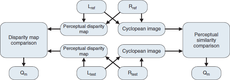
Figure 7.9 Block diagram of the 3D quality metric [90].

There are several other 2D to 3D metrics proposed and these include the following metrics:

1. Hewage et al. [91] compare the results of subjective tests with the 2D VQM score of stereoscopic videos encoded with a depth-image-based representation. The comparisons show that the scores have high correlation with both the overall perception of image quality and depth perception from the subjective studies. This shows the possibility of using VQM for evaluating 3D images.
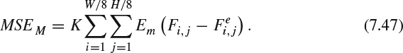
2. Benoit et al. [92] propose to enhance SSIM for depth maps using a local approach for the measure of the disparity map distortion in order to extend 2D metrics to 3D perceptual metrics. A block diagram of the local approach for SSIM is given in Figure 7.10.
3. Gorley et al. [93] propose stereo band limited contrast (SBLC) for evaluating stereoscopic images using two-view conventional video streams. The metric first uses the scale invariant feature transform (SIFT) [94] to extract and match the feature points in the left and right views. Then, RANdom SAmple Consensus (RANSAC) [95] is applied to these features for searching the matching regions between the left and right views. The matching regions are used to calculate HVS sensitivity to the contrast and luminance impairments. Finally, the HVS sensitivity is used for the perceptual score.

   

   Figure 7.10 Block diagram of the proposed 3D metric using local approach for SSIM [92].

4. Shao et al. [96] propose a metric for the quality of stereo images encoded in the format of depth-image-based representations. The metric consists of two parts: the color and the sharpness of edge distortion (CSED) measurement. Color distortion is a fundamental 2D measurement for the comparison in luminance between the reference image and test image. The sharpness of edge distortion is calculated based on the edge distortion in the test image weighted with the depth in the original image. Both measurements are combined by a weighting average of both measurements to give the score as the quality metric of the stereo image.
5. Yang et al. [97] propose a method to measure the quality of stereo images encoded in the format of image-based representations using the 2D image quality metrics in the stereo sense. The image quality is calculated as the mean of PSNRs of the left and right images respectively, and the stereoscopic evaluation is then adjusted according to the absolute difference between stereo images.
6. Lu et al. [98] propose a metric for mixed-resolution coding 3D videos using a spatial frequency dominance model. A weighted sum of differences and imparities in spatial frequencies between the test image or video and the reference image or video is calculated to represent the perceptual quality.

7.2.3.2 Why 2D Metrics Fail for 3D Images

The simplest scenario to extend 2D metrics to 3D metrics is to calculate the mean of 2D metrics from the two views independently, which is used as the stereoscopic perceptual score. The assumption for this scenario is that impairments in each view have equal effect on the perception of stereo videos but this assumption fails in many cases. This is similar to the condition when using the mean quality over all individual frames in a video because the video metric cannot reflect the effects in temporal masking and thus separate evaluations in both views fail to predict the inter-view masking effects in stereoscopic vision. Although the difference between two views of a point in the scene is an important depth cue for the HVS and the HVS can fuse this difference into a single 3D image, artifacts in both views may introduce a contradiction in binocular depth cues and cause serious distortions in 3D stereoscopic perception. Several different theories discuss the effects of impairments on the HVS perception but generally also believe that the view perceived by one eye may suppress the view perceived by the other eye instead of fusing the contradictory cues. This phenomenon is called binocular suppression theory which illustrates the masking and facilitation effects between the images perceived by each eye [99]. This is similar to the temporal masking effects in video. The subjective study in mixed-resolution coding [100] shows that the overall perceived quality is closer to the quality of the better channel instead of the mean of the quality of both views. Furthermore, the content in the video also affects the 3D perceptual quality. The extended 2D metrics fail to accurately measure the 3D quality metrics because they fail to model the perception of human stereoscopic vision. There are two important properties which must be considered when designing a 3D quality metric:

1. The model should consider the quality of the cyclopean image and binocular disparity of the scene separately. The degradation in the cyclopean image is perceived as 2D distortions and the degradation in the binocular disparity is perceived as 3D distortions.
2. Because the HVS perceives the fused results instead of individual artifacts in each channel, the cyclopean and binocular perception of the distortions may affect each other but the effect is generally nonlinear as shown in the following ways:

   (a) Pictorial depth cues are important for the depth perception. In addition there are masking and facilitation effects between depth cues coming from the two perception models. Therefore, the perception quality of binocular disparity is affected by the cyclopean image perception. Past studies [101, 102] show that motion parallax and stereopsis are considered more important depth cues over monocular depth cues such as shadows, texture, and focal depth. Furthermore, blur is perceived mainly as a “2D” distortion and affects the cyclopean image rather than binocular disparity. The subjective studies [101] also verify that the quality of the cyclopean image might have some distortions and the perception of depth might still be perceived perfectly under minor distortion. However, as the cyclopean quality drops further beyond minor distortions, the accuracy of depth perception drops accordingly. The results correspond to the study results [33, 30] which claim that the depth effect only contributes to the quality perception when there is little compression. This effect suggests that there is an influence of 2D artifacts over the 3D perception.

   (b) Cyclopean perception is affected by the scene depth. The masking in the cyclopean view during image fusion may relieve the artifacts on the cyclopean perception. Therefore, the cyclopean image perception is affected by the perception quality of the binocular disparity. The stereoscopic depth modifies the perception of image details. Boev et al. [101] and Kunze et al. [33] show that equivalent information loss of image fidelity in videos is perceived very differently in 2D and 3D videos. The subjective studies [101] show that the binocular disparity affects the cyclopean image perception in two different ways depending on changes in local or global binocular disparity. Generally, local binocular disparity affects the convergence of the eye and in turn determines which image regions are fused together in the cyclopean image and this therefore has an effect on the region of the cyclopean image comparison and on distortion detection. Global binocular disparity changes the perceived volume of the 3D scene. A larger variance of disparities in the stereoscopic pair generates the perception of a more spacious scene. Thus, Kunze et al. [33] showed that the presence of depth affects the perception of the image quality.

According to these observations, 3D stereoscopic perception metrics, as shown in Figure 7.11a should be designed in the following steps:

1. Extract the cyclopean image and binocular disparity from both the test video and reference video.
2. Evaluate the quality scores separately in each format according to the first property discussed above.
3. Design a measurement function to compute the final metric using the quality score in each format when taking into account mutual influences in both channels according to the observation of the second property discussed above.

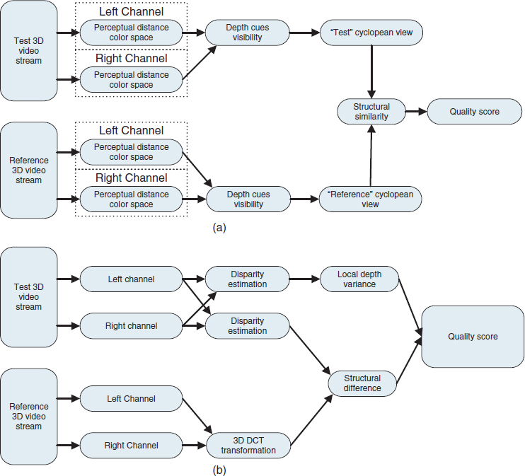
Figure 7.11 Image processing channel for 3D quality estimation: (a) comprehensive model for offline processing, (b) simplified model optimized for mobile 3D video.

Traditional optimized 2D video quality metrics can be used for comparing the quality of the cyclopean images. However, adequate knowledge about the mutual effects of the cyclopean image and binocular disparity on the perception of each other is required. Proper subjective tests have to be designed for these investigations, too. The following will present a set of metrics based on the steps discussed in the previous paragraphs.

7.2.3.3 Real HVS 3D Video Metrics

Subjective studies [101, 103] show that binocular fusion and binocular difference are two important prospects in binocular disparity. The original binocular disparity model can be simplified to focus on binocular fusion and depth extraction processes and compute contrast sensitivity in the frequency domain as shown in Figure 7.11b. The quality score is computed by comparing two DCT video streams. The binocular convergence is performed by searching for similar blocks in the left and right views, and the binocular fusion in lateral geniculate nucleus (LGN) is modeled by a 3D-DCT transformation over similar blocks in the left and right views. DCT simplifies the computation and comparison among patches in different spatial frequency and orientation for estimating the pattern masking and CSF. The perception of depth is estimated by calculation of disparity between the views in the test video stream with the help of local depth variance. Direct comparison of disparity between the test video stream and the reference video stream induces errors in metrics estimation and cannot reflect the perception of depth. Thus the algorithm compares the cyclopean distortion between the test video stream and the reference video stream but only computes the depth perception in the test video stream, and the depth is used as a weight for the output score because binocular depth is only a relative cue. The disparity variance matters most and is calculated on a local area of angular size of one degree corresponding to the area of foveal vision. Larger disparity variance generally represents more obviously perceived depth. The following are three different methods for considering these effects:

1. 3D Peak signal-noise-raito based on human visual system (PHVS-3D) stereoscopic video quality metrics

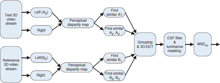
   The PHVS-3D metric [103] is given in Figure 7.12. The test video and the reference video consist of a stereo-pair view. The depth perception from two views is manifested as a disparity map. Both the test video and the reference video are fed in to compute the disparity map between the corresponding left and right video streams. The algorithm runs the assessment on blocks. As shown in Figure 7.12, for each reference block A₀ in the left view of the test video stream, the algorithm locates the matching block B₀ in the left view of the reference video stream and the most similar blocks which are A₁ in the left view and A₂ and A₃ in the right view in the test video streams. B₀ is used to locate the most similar blocks which are B₁ in the left view and B₂ and B₃ in the right view in the reference video stream. All similar blocks are located in a 3D structure and all blocks are transformed to the 3D-DCT domain. All 3D-DCT transformed blocks are corrected with luminance masking and the contrast sensitivity function. The mean square error between the 3D-DCT test block and the reference block is computed for measuring the stereoscopic video quality. The following are the key elements for execution of this algorithm:

   

   Figure 7.12 Flow chart of the PHVS-3D quality assessment model.

   (a) Finding the block-disparity map: The disparity (or parallax) is shown as the difference between the left view and the right view of the same 3D point in the scene, and the value is generally inversely proportional to the depth of the point, as discussed in Chapter 2. Generally the disparity is computed using a stereo matching algorithm, as discussed in Chapter 4. The dense disparity map between the left view and the right view is computed using the block matching algorithm [104] with a block size of 9 × 9.

   (b) Block selection and 3D-DCT transform: The DCT basis method can de-correlate data and achieve a highly sparse representation and thus is used to model two HVS processes:

   i. The binocular fusion process [105]

   ii. The saccades process which is pseudo-random movement of the eyes for processing spatial information [106]

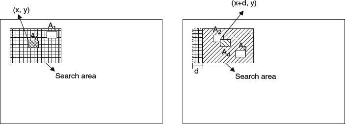
   The DCT basis consists of all these similar blocks stacked together and can be used to explore the similarity across views and in the spatial vicinity. The similar blocks to the base blocks A₀ and B₀ in the left view and right view from the test and reference videos are found by using block matching (BM). BM searches the left view and right view to find the best matched block in the left view and two similar blocks in the right view as shown in Figure 7.13. A₀ is the base block and A₁ is the similar block in the left view. A_d is the corresponding block with a disparity of d. A₂ and A₃ are the best matching blocks to A₀ in the search region of A_d. A = A₀, A₁, A₂, A₃ and B = B₀, B₁, B₂, B₃ are respectively the four blocks in the reference stereoscopic image and test stereoscopic image. Then 3D-DCT is applied to A and B respectively. Jin et al. [103] chose a 4 × 4 block size and a 28 × 28 searching region for this metric.

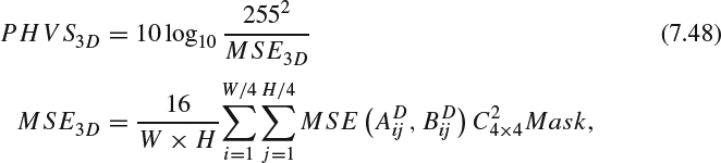
   (c) Modified MSE: The metric extends PSNR-HVS [73] and PSNR-HVS-M [74] to compute a modified MSE for considering contrast masking and also between-coefficients contrast masking of DCT basis functions in a block size of 4 × 4. The coefficients of the top layer in the 4 × 4 × 4 3D-DCT block which represents the concentration of most energy are weighted with a masking table [74]. Other layers are weighted with coefficients computed from the energy distribution of the block. The PHVS-3D can be computed as:

   

   Figure 7.13 An example of block selection in stereoscopic image.

   

   where W and H are the width and height of the image, is the first layer of 4 × 4 × 4 3D-DCT coefficients indexed at the left-top corner of location [4i, 4j] in the reference image, is the corresponding one in the test image, C_4×4 is a correcting constant determined by the CSF [73] and Mask is the contrast masking correction constant [74].

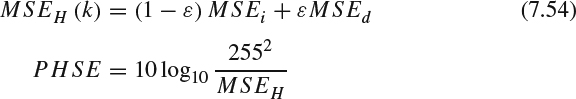
2. PHSD 3D video quality metrics

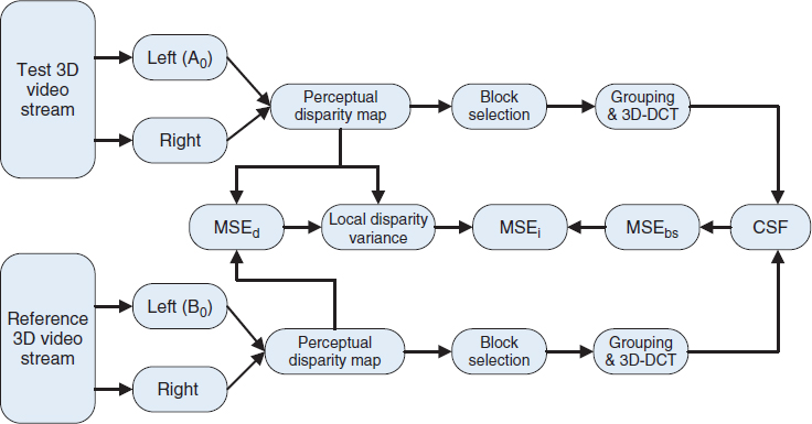
   Figure 7.14 shows another stereo assessment method which extends the concept of PHVS-3D [103]. The disparity maps are first computed from the test image and reference image. The mean square error (MSE) of the difference between the reference disparity map and test disparity map is calculated and denoted as MSE_d, and the local disparity variance of the reference is also computed to model the depth perception. A similar 3D-DCT transform to that used in PHVS-3D is applied to the test and reference images. Both 3D-DCT transformed structures are modified to consider the effect of the contrast sensitivity function. The MSE of the difference in the 3D-DCT coefficients is computed to represent the cyclopean perceptual difference in the DCT domain and is denoted as MSE_bs. The local disparity variance of the reference image is used to scale MSE_bs according to the ability of detecting distortions on flat areas or pronounced-depth regions. The detail of the key steps for the algorithm are presented in the following:

   

   Figure 7.14 Flow chart of the PHSD-3D model.

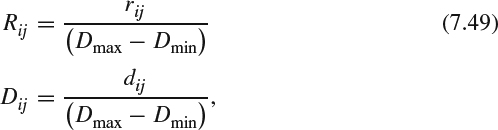
   (a) Local disparity variance: PHSD-3D suggests that the disparity should be normalized with the disparity range of the target display. Boev et al. [107] and Hoffman et al. [108] proposed that the disparity range represents the comfort zone and is defined in terms of cm or the number of pixels for the target display with respect to the Percival's zone of comfort [108]. The disparity is normalized as:

   

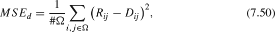
   where r_ij and d_ij are the estimated disparity at the location [i, j] in the test image and reference image respectively, D_max and D_min are the minimum and maximum disparities of the comfort zone in number of pixels. The MSE of the global disparity differences between the reference disparity map and test disparity map is computed as:

   

   where Ω is the domain which contains all the pixels in the entire image whose disparity can be confidently estimated, that is, the pixel in the left can find its corresponding pixel in the right, and #Ω is its cardinality. Those pixels from the left that cannot find corresponding pixels in the right are marked as holes and are excluded from the estimate.

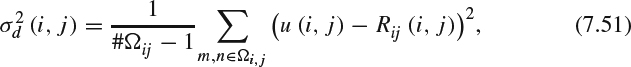
   The local disparity variance is computed inside a W_f × H_f block where W_f and H_f are used to approximate the size of the fovea projected to the screen in the typical viewing distance, and the fovea block is identified by its center pixel index. For example, the proper block size for a mobile 3D display may be chosen as 28 × 28. The local variance can be computed as:

   

   where u(i, j) is the mean disparity calculated over Ω_i,j inside the fovea block [i, j] and Ω_ij ∈ Ω are those pixels whose disparity can be estimated confidently inside the fovea block at [i, j]. The local variance value models the variation of depth around the central 4 × 4 block around the pixel [i, j] and can be used to correct the visual impairment induced by binocular disparity.

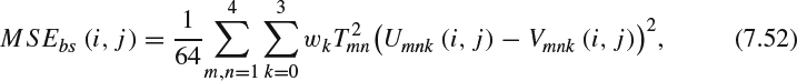
   (b) Assessment of visual artifacts in a transform-domain cyclopean view model: After applying 3D-DCT transformation at a pixel [i, j] as described previously, the 3D-DCT coefficients are passed through a block which models the CSF and masking effects at that pixel in the following manner:

   

   where U = U_mnk(i, j), m, n = 1 … 4, k = 0 … 3 and V = V_mnk(i, j), m, n = 1 … 4, k = 0 … 3 are the 4 × 4 × 4 DCT coefficients at the pixel [i, j] for the test and reference image respectively, w_n is the weight of the nth layer and T_mn is the CSF masking coefficient which represents the masking effect for each layer and is scaled down by a factor determined by the energy distribution for each transform layer.

   (c) Weighting with local disparity variance: Subjective studies [103] show that the distortions are more obvious in the flat regions than in pronounced-depth regions such as edges when the distortion is low. However, when the distortion is high, the presence of depth did not affect the perceived quality. Therefore, the metric makes two assumptions:

   i. The high disparity region represents the place where the depth is highly pronounced.

   ii. The structural distortions are less visible in highly depth-pronounced regions if the distortions are below a threshold.

   The local disparity variance should correct the perceptual error estimation MSE_bs(i, j) at [i, j] as follows:

   

   Then, MSE_i of the image is calculated as the average of MSE_3dbs over all pixels.

   (d) Composite quality measure: The overall assessment should be a combination of MSE_i and MSE_d and then transformed from error to PSNR-type measurement:

   

7.2.3.4 Feature-based 3D Video Quality Evaluation

Although a feature-based method already takes image structure into account, a 3D feature-based method should be 3D model aware. Figure 7.15 illustrates the possible stages of stereoscopic vision for a 3D feature-based metric. The view of a scene is first collected by each eye through the photo receptors on the retina. The processing in the retina is responsible for the luminance masking, color processing and contrast sensitivity as discussed in Section 7.2. Then the information is passed to the LGN, which mainly focuses on binocular masking and extraction of binocular depth cues. Then the single and fused information is sent to the V₁ visual center in the cortex. V₁ is responsible for the spatial decomposition and spatial masking with different spatial frequencies and orientations. Finally, temporal masking follows. In addition, a small part of the visual information is directly fed to the V₁ cortex without being processed in LGN according to the binocular suppression theory and anatomical evidence. The depth perception occurs in the higher and later processes after V₁. Thus the process shown in Figure 7.16 which simulates the process in Figure 7.15 makes possible masking and facilitation effects between depth cues. The presence and strength of one type of depth cue might suppress or enhance the perceptibility of another. This makes the process of estimating depth cues and binocular masking together necessary.

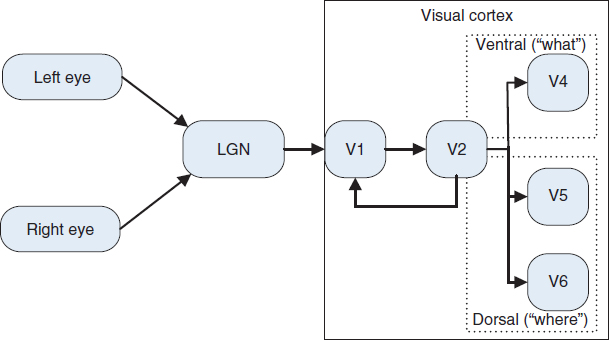
Figure 7.15 Modeling of the stereoscopic HVS in 3D vision process.

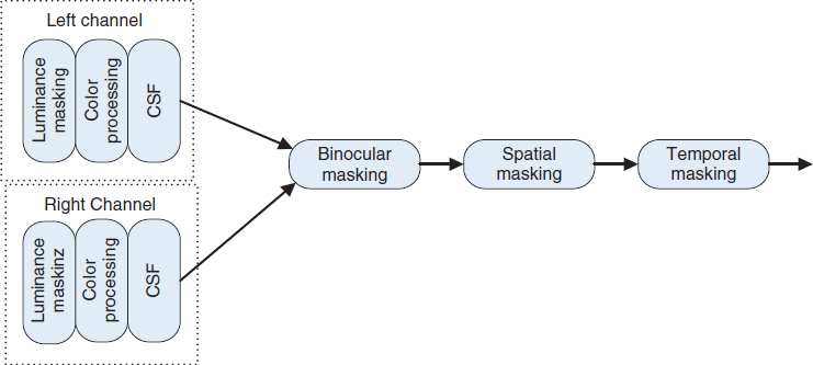
Figure 7.16 Modeling of the stereoscopic HVS using image processing channel realizing the 3D vision process.

When the expected artifacts are limited and the amount of computation for metrics is also constrained, feature-based quality estimation is more suitable than HVS-based quality estimation. Figure 7.17 shows a model-aware feature-based 3D quality metric. The inputs are two 3D video streams: test and reference. First, each video is transformed into a perceptual color space using methods such as S-CIELAB [109] and ST-CIELAB [110]. Then, the visibility of depth cues and the suppression among different depth cues are calculated and recorded as 3D quality factors. An optional block such as [59, 71] can be used to estimate the temporal integration and masking. Finally, the derived cyclopean view and perceptual disparity map are formed from the cyclopean view and compared by a structural similarity metric, which estimates CSF and perceptual salience of different areas in the visual content to form the indicator of 2D quality. Good structural similarity algorithms include [58] which is based on local statistics and [89] which uses adaptive scales. At the end, the final quality measure should be computed using a nonlinear weighting function to combine the 2D and 3D quality measurements:

Figure 7.17 Image processing channel for feature-based quantity estimation.

where f_depth describes the influence of binocular disparity over the cyclopean perception and f_cues describes the influence of cyclopean distortions over the depth perception.

7.2.4 Postscript on Quality of Assessment

Although video quality assessment on traditional 2D video has been an active research topic and has reached a certain level of maturity [111], 3D video quality assessment is still in its early stages and remains an open research direction (see an early survey of 3D perceptual evaluation [3]). The works [112, 113] extend the well-established 2D video quality measurement methods for 3D scenarios and indicate that certain 2D measurements on the left and right view can be combined together to evaluate the 3D stereoscopic quality. However, in many cases a stereo video exhibits different characteristics from 2D video systems and provides dramatically dissimilar viewing experiences such as the perception of accommodation, binocular depth cues, pictorial cues, and motion parallax. Moreover, the compression/rendering approach also affects the quality assessment scheme. More customized quality assessment methods are expected to address the uniqueness of different codecs [114].

For free viewpoint video systems, the quality assessment can be additionally quantified as the structure error in reproducing the appearance of a scene, because the human visual system (HVS) is good at perceiving structural and temporal details in a scene, and errors in features or geometric structure are prominent. The accuracy of a synthesized image is quantified as the registration error with respect to a reference image using the 90th percentile measure of Hausdorff distance [18]. This framework provides a single intuitive value in terms of pixel accuracy in view synthesis to evaluate free viewpoint 3D video system. However, the quality metrics for stereoscopic and free viewpoint video systems are still open problems and active research topics.