10.1 Rate Control in Adaptive Streaming

Streaming 3D video over communication networks for real-time application has many challenges. One of these is how to utilize the current limited network resources to achieve the best perceived 3D video quality. Besides, the bandwidth provided by the network may vary from time to time. For the best received quality, the streaming applications need to dynamically perform rate control to adjust the encoding rate at the encoder side to fit in the current network status and maintain the playback smoothness at the decoder side. However, different coding tools and modes can be selected to meet the same target bit rate but result in different perceived quality. Although the encoder can resort to the full search methodology by trying all possibilities for best tradeoff, this kind of solution is often NP hard and/or very time consuming, thus not practical for real-time applications. It is desired to have a fast selection method for near-optimal solutions to reduce the computation complexity at the encoder side. In this section, we will address both the rate control and the mode decision issue in the 3D video streaming applications.

10.1.1 Fundamentals of Rate Control

A generic 3D video streaming framework is shown in Figure 10.1. The encoder located at the transmitter side will adjust the coding parameters to control the bit rate according to the latest estimated network bandwidth and optional error control message through receiver's feedback. The decoder located at the receiver side equips a decoder buffer to smooth out the network jitter and the bit rate fluctuation owing to different coding parameters being selected by the encoder. The main objective of the decoder buffer is to ensure that the playback is as smooth as possible. As we can see from Figure 10.1, there are two common constraints that the encoder needs to follow so that the playback at the decoder side can be smooth. The first constraint is that the bit rate sent from the transmitter should not exceed the capacity of the underlying networks at any time instant. Without any buffering mechanism deployed at the transmitter side, those out-of-capacity bits will be dropped out and cause decoding problems at the decoder side as video streams exhibit strong decoding dependency. The second constraint is the fullness of the decoder buffer: it should neither underflow, which causes playback jitter, nor overflow, which drops bits which causes video quality degradation and error propagation.

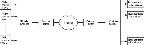
Figure 10.1 Framework of 3D video streaming.

Given the aforementioned constraints, the encoder needs to adjust the encoding parameter such that the perceived video quality is as high as possible. A well-known rate control method for traditional 2D video is defined in MPEG-2 test model 5 (TM5) [1]. Basically, TM5 rate control follows a top-down hierarchical approach and consists of three steps: (1) target bit allocation at frame level by addressing the picture complexity in the temporal domain; (2) rate control at macro-block (MB) level by addressing the buffer fullness; (3) adaptive quantization to refine the decision made in step (2) by addressing the varying texture complexity in the spatial domain. The bit allocation is assigned by a complexity model according to different inter/intra type: I, P, or B. Consider the scenario that the channel bandwidth is R bits per second (bps) and the picture refresh rate is F. An N-frame group of pictures (GOP) consists of N_I I-frames, N_P P-frames, and N_B B-frames: N = N_I + N_P + N_B.

In the first step, the encoder allocates bits to N frames within a GOP with N frames such that the overall number of bits consumed in one GOP is NR/F. The complexity model assumes that the number of bits for one frame multiplied by its quantization scale remains around a constant, and has the following expressions:

where X, S, and Q represent the complexity, number of bits for one frame, quantization scale, respectively, and the subscript denotes the different picture type. The complexity is first initialized before the encoding as:

After encoding the first frame for each type, the complexity model of each picture type in (10.1) is updated according to both the average chosen quantization scale and the number of bits consumed.

To provide consistent perceived video quality across different picture types, empirical studies suggest that it can be achieved by setting a constant ratio between different quantization scales. In other words:

where the value of K_I, K_P and K_B are suggested to be 1.0, 1.0, and 1.4 in TM5. Bringing in (10.3) to (10.1), the number of bits for each picture type can be rewritten as:

Note that the targeted total number of bits allocated in a GOP is to achieve NR/F:

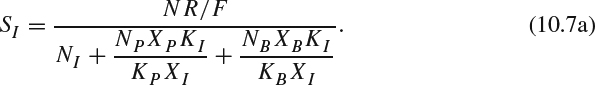
The number of bits for I type, S_I, can be derived as follows. By rearranging (10.4), S_P and S_B can be represented by S_I:

By combining (10.6) and (10.5), we arrive at:

Similarly, we can have S_P and S_B as:

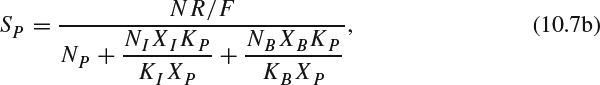
and

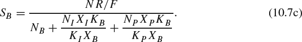
After allocating bits in the frame level, in the second step, the bits are allocated in the MB level by adjusting the reference quantization scale for each MB with the consideration of buffer fullness. For the j th MB, the reference quantization scale, Q_j, is computed as:

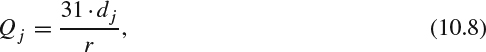
where d_j is the decoder buffer fullness, and r is a reaction parameter defined as r = 2R/F.

It is often noticed that the spatial complexity within a frame is not a constant and varies from one region to another, depending on the local texture and activities. The activity factor, act_j, is obtained by first calculating the variances of all luminance 8×8 blocks within one 16×16 MB, selecting the minimum variance among all candidates, and adding a constant value, one, to the selected minimum variance. The activity measurement will be normalized as:

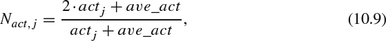
where ave_act is the average act_j in the previous picture. For the first frame, ave_act is set to 400. The final used quantization scale will be refined by addressing the local activity measurement, N_act,j, and can be calculated as:

The rate control method in MPEG-4 verification model (VM) is an extension of MPEG-2 TM5 but with a more precise complexity model [2]. Denote the number of bits for one frame as S and the number of bits for nontexture information, such as header and motion vectors as H, and the mean of absolute difference (MAD) computed using motion-compensated residual for the luminance component as M. The R–D curve is described by a quadratic model:

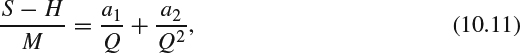
where a₁ and a₂ are the first and the second order coefficients and can be estimated on-line via the least squared solution.

A similar top-down bit allocation strategy from GOP-level, picture level, to uniform slice level is adopted in H.264 JM software (JVT-G012) [3]. Note that H.264 does not define a picture as a pure I/P/B-frame type since a frame can contain I/P/B slices. The complexity model (X_I, X_P, and X_B) used in MPEG-2 and MPEG-4 is replaced by the concept of signal deviation measure σ for each frame in H.264 codec. The signal deviation measure will be updated by the first order polynomial predictor from the MAD of the previous stored picture. The main goal of the GOP level rate control is to control the deviation of the quantization parameters in a small range from one GOP to another, such that the video quality fluctuation is maintained under an unnoticeable level. The decoder buffer occupancy should be checked to avoid overflow and underflow. There are two stages in the picture-level rate control: pre-encoding and post-encoding. The pre-encoding stage is to calculate the required quantization parameter for each picture, and the post-encoding stage is to refine the quantization parameters for each uniform slice or MB unit by the given allocated bit rate. The quadratic R-D model (10.11) is used. At the MB-level, a rate distortion optimization (RDO) strategy is deployed by formulating the rate control problem as minimizing the overall distortion subjected to a given target bit rate by selecting the coding method. The general RDO process is constructed as follows. Denote s_k as the kth coding block and s = [s₀, s₁, …, s_{K − 1}] is the collection of all coding blocks in one MB. Denote m_k as the selected mode in the kth coding block and m = [m₀, m₁, …, m_{K − 1}] is the collection of all coding modes in one MB. The distortion and the bit rate are functions of selected coding modes and they can be represented as D(s,m) and R(s,m), respectively. With a maximal bit rate budget, R, the optimization problem is formulated as:

This constrained optimization problem can be reformulated as an unconstrained optimization by introducing a Lagrange multiplier, λ. The objective function becomes:

With a given λ, we can have a corresponding optimal solution of (10.13). The optimal solution of (10.12) is achieved when the selected λ results in R(s, m) = R. For simplicity, the overall distortion function within an MB is assumed as independently summed from each coding block. The objective function can be decomposed intok small functions and can be solved individually.

More specifically, the formulation in JM H.264 is to optimize the following cost function by selecting the optimal coding mode under a given quantization parameter, Q_P, and the value of associated λ_MODE:

where MODE can be the intra-prediction mode or the inter-prediction mode. Let s(x, y, t) be the original pixel value with coordinate (x, y) at frame t and let A be the collection of coordinates for all pixels in the considered coding block. Depending on whether intra or inter mode is selected, the distortion and the λ_MODE are calculated differently.

For intra mode, the distortion, D_REC, is measured as sum of squared difference (SSD) as follows:

where s_INTRA(x, y, t)is the pixel value after intra mode coding.

For inter mode, the distortion measurement, D_REC, is calculated as the displaced frame difference (DFD):

where (m_x, m_y) is the motion vector pair, s_INTER(x − m_x, y − m_y, t − m_t) is the pixel value after inter mode coding, and p as the coding parameter to choose different order of distortion.

λ_MODE is suggested from the experiment as follows:

Depending on the chosen order of inter-mode distortion measurement, λ_INTER has a different expression:

10.1.2 Two-View Stereo Video Streaming

The rate control for two-view stereo video rate control can be extended from previous discussed methods according to the adopted stereo video codec. For the individual view coding, which encodes left view and right view with two independent video encoders, one could deploy the joint multi-program rate control method commonly used in multiuser scenario [4, 5]. Although the bit streams are encoded independently in the individual view coding scenario, the underlying resources, such as bit stream buffers and allocated transmission channels, can be merged together and jointly utilized to achieve higher multiplexing gain. Besides, the encoder can further explore the diversity gain exhibited from different content complexity via (10.1) or (10.11) in both views, and allocate bits to each view accordingly.

For the frame-compatible stereo video streaming, one could deploy and extend the commonly used single-program rate control method. Note that each picture in the frame-compatible stereo video contains two downsampled views. Advanced rate control methods to address different characteristics of these two different downsampled views can be used for better visual quality. For example, if TM5 rate control method is used, the average spatial activity measurement, ave_act, used in (10.9) may need to have two variables to track regions in two different views. For the full-resolution frame-compatible stereo video streaming, the codec has one base layer and one enhancement layer. The enhancement layer has decoding dependency on the base layer. The scalability and dependency often bring a penalty on coding efficiency [6]. Given a total bit budget for both layers, different rates assigned to the base layer and enhancement layer will result in different perceived quality in the base layer only and in the base layer plus enhancement layer. A balanced bit allocation between two layers can be performed for different video quality requirements from the baseline half-resolution experience and enhanced full resolution experience.

As discussed in Chapter 5, the binocular suppression theory suggests that the video qualities measured by objective metrics, such as PSNR, in both views do not have a strong correlation to the perceived stereo video experience. Based on this observation, the bit allocated in the dominant view can be higher than that of the non-dominant view.

10.1.3 MVC Streaming

The MVC codec encodes one more dimension to incorporate different camera views. A group of GOP (GGOP) from multiple views is often constructed first. A straightforward method for MVC rate control is to start the bit allocation from this GGOP level. After allocating bits to each view, one could employ the common 2D video rate control scheme to handle the frame level and the MB level. In [7], the bit budget allocation for each view is based on the view complexity measured by the correlation between the base view and the predicted views. Denote I(x, y, v) as the (x,y) pixel located at the v-th view and the dimension for each view is W × H. The correlation between view v and base view 0 is calculated as:

where

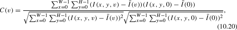
The correlation will be normalized as:

Given a total bit rate, R, for one MVC stream, the rate allocated to view v, R_v, will be:

The correlation-based bit allocation will assign more bits to the views with higher similarity to the base view, thus the summed distortion over all views is minimized. When equal video quality among all views becomes a requirement, one can modify the weighting factors, {w(v)}, by assigning more bits to the views with lower correlation. In that regard, the system's objective becomes to maximize the minimal video quality among all views [8].

An RDO approach can also be adopted in the MVC streaming rate control by searching the quantization parameter in each view [9]. Similar to the independent optimization methodology used in H.264 optimization, the optimization problem can be decoupled to several subproblems and solved independently via a trellis expansion.

10.1.4 MVD Streaming

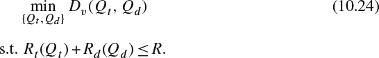
In the MVD coding, some views are not encoded in the bit streams and need to be synthesized from neighboring texture videos and depth maps. Therefore, the visual quality of the synthesized view, D_v, depends on the quality of the reconstructed texture videos and depth maps from the neighboring coded real views. The distortions of those coded real views depend on the selected quantization parameters. One can simplify the problem to reduce the range of parameters set by assuming that both neighboring coded real views use the same quantization parameter to achieve similar perceptual quality. Denote Q_t and Q_d as the selected quantization parameter for the texture video and depth map in both neighboring views, respectively. Then, D_v can be expressed as a function of Q_t and Q_d, namely, D_v(Q_t, Q_d). The required bit rate in the texture video, R_t, and the depth map, R_d, can be also expressed as functions of quantization parameter Q_t and Q_d. In other words, the rate functions are R_t(Q_t) and R_d(Q_d). The major issues in MVD streaming are how to distribute bits to the texture videos and depth maps, given a total rate constraint, R, so that the perceived video quality at the desired viewing position(s) is optimized. One can formulate the bit allocation in MVD streaming application to optimize the synthesized view's distortion by selecting the optimal Q_t and Q_d in both neighboring real views subject to the rate constraint, R:

A full-search method can be conducted to find the optimal encoding parameters in both texture and depth video at the cost of higher computation complexity [10]. The full-search is performed on the 2D distortion surface constructed by one dimension along the texture video bit rate and another dimension along the depth map bit rate. Although the optimal solution can be found from a full search methodology, the computation complexity is often very high. A distortion model for the synthesized view is often desired such that the computation complexity can be simplified [11].

Since the synthesized view is often generated from a linear combination of neighboring real views, the distortion of the synthesized view can be modeled as a linear combination of the distortion from texture image and depth image belonging to both neighboring left view and right view [12]:

where , , , and represent the compression distortion for the reconstructed left view texture video, right view texture video, left view depth map, and right view depth map, respectively. α_L, α_R, β_L, β_R, and γ are the model parameters and need to be estimated.

Since the video's encoded rate and distortion are functions of the selected quantization parameters, the encoded rate for texture, R_t, and depth, R_d, in both neighboring coded views can be modeled as functions of the corresponding quantization step as follows:

where a_t, b_t, a_d, b_d are the rate-quantization model parameters and need to be empirically estimated. The distortion for texture, D_t, and depth, D_d, in both neighboring coded views can be modeled as functions of corresponding quantization step:

where m_t, n_t, m_d, n_d are the rate-quantization model parameters and need to be empirically estimated. With the assumption that the content in both neighboring coded views is similar, the distortion in the neighboring views is very similar by using the same quantization parameter. Therefore, the distortion in the synthesized view, D_v, can be further simplified and modeled as a function of Q_t and Q_d in both views.

Having those models, problem (10.24) can be reformulated as:

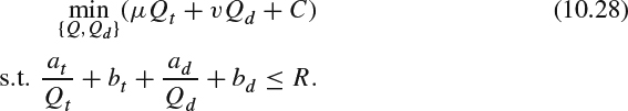
Standard optimization methods, such as the Lagrangian multiplier method, can be applied to solve Q_t and Q_d.

With a model to describe the rate-quantization and distortion-quantization relationship, one can apply it to the MVD rate control. In [13], the rate control is conducted via a top-down approach by first assigning a bit rate for each real view, then allocating bits between texture video and depth map in each view, and finally conducting frame level rate allocation. In the frame level rate allocation, the quantization parameter is adjusted to satisfy the decoder buffer fullness requirement. Similar to most rate control methods, the distortion-rate-quantization model needs updating after a frame is encoded.

When the number of views becomes large in the MVD case, one may choose to transmit fewer coded views to save on bit rate. In this scenario, several intermediate views need to be synthesized between two neighboring coded views from the bit streams. An important question is how to select the most important views to be encoded in the streams and leave other views to be synthesized at the rendering stage so the overall distortion from all views are minimized subject to a target bit rate. As the distance between these two neighboring coded views is large, the selected quantization parameters will be different to address different content complexity owing to different viewpoints. Under this condition, the distortions in these two neighboring coded views are not similar. Consider a synthesized view at a virtual viewpoint having a distance ratio to the left coded view and the right coded view as k/(1−k), where 0 ≤ k ≤ 1, the distortion of this synthesized view can be modeled as a cubic function with respect to the viewing position between two coded real views [14].

The parameters c₀, c₁, c₂, and c₃ can be estimated from curve fitting technology such as least squared solution by sampling a small number of virtual views and synthesizing the view to measure the distortion. With this more general model, we can formulate a more generalized problem to minimize the overall distortion in all coded views and the synthesized views subject to the rate constraint by: (1) selecting which views to code and which views to synthesize and (2) choosing the quantization parameters for texture video and depth map in the coded view. The optimal solution can be found using the 3D trellis algorithm.