6.2 Wireless Communications

The subject matter of this book relates to the transmission of a digital data over a wireless channel. Several stages of processing are needed in order to do this. All these stages, along with the information-generating source and the channel itself, are seen as a wireless communications system. Often, an ease of analysis dictates that the system is considered with a simplified structure that includes only the main blocks. These blocks are in the sequential order during transmission and assuming that the source is already in a digital form,

• In the transmitter:
  • Source encoder: This block is concerned with the representation of the information from the source, usually appearing as a group of samples organized in a source data block, in digital form (as a sequence of bits). The most important operation that is performed in the source encoder, in what concerns this book, is the representation of the information from the source in a compact and efficient way that usually involves compression of the source data block.
  • Channel encoder: This block protects the sequence of bits from the source encoder against the errors that the wireless channel will unavoidably introduce. This is done by adding extra redundant bits and a specific structure to the sequence of bits that is presented to the input of the encoder. Because this operation adds redundant bits, the number of bits at the output of the channel encoder is never less than the number of bits at the input. The ratio between the number of bits per unit time at the input of the encoder to the number of bits per unit time at the output to the encoder is called the channel code rate. Following its definition, the channel code rate is always less than or equal to one.
  • RF (radio frequency) transmit side: In this stage the digital signal to be transmitted is converted into an analog electrical signal able to travel as an electromagnetic wave. Some of the operations included in this block are modulation and power control.
• Between transmitter and receiver:
  • Channel: The medium over which the electrical signals are transmitted as electro-magnetic waves. The study of the characteristics of the wireless channel will be discussed later on in this chapter.
• In the receiver:
  • The blocks in the receiver are the complement of those at the transmitter, in the sense that they perform the reverse operations performed at the transmitter so as to ideally obtain at the output of the receiver the same group of samples as at the input of the transmitter.

Next, we discuss further details about some of these components of a wireless communications system. More detailed information on these topics can be found in the many very good existing textbooks on networking, such as [5], [6] and [7].

6.2.1 Modulation

As summarized in the previous paragraphs, in order to transmit digital data over a wireless channel it is necessary to perform several stages of signal processing before the actual transmission of the information over the wireless channel. While most of these operations are preferably implemented in the digital domain (and over several protocols organized in layers), it is eventually necessary to convert the stream of bits into an analog electrical signal that can travel as electromagnetic radiation over the wireless channel. This operation, performed at the physical layer, is called modulation. In order to be able to communicate information, modulation maps the data bits to be transmitted into variations of an electrical signal. These variations, which are referred as the operation of modulation, usually take the form of changes in amplitude, phase or frequency in a sinusoidal electrical signal:

where the signal ϕ(t) includes both the changes in frequency f(t) and in phase θ(t) because ϕ(t) = 2πf(t)t + θ(t), α(t) is the variation in amplitude, f_c is the carrier frequency, ϕ₀ is an initial phase (which often can be considered equal to zero without loss of generality), and T_s is the duration of the symbol in the equation. Using trigonometric properties, the above data-modulated sinusoid can also be written as:

There are multiple types of modulation scheme, each differing in how the bits are mapped and what sinusoid parameters are actually modulated. Some of the most popular ones are summarized next.

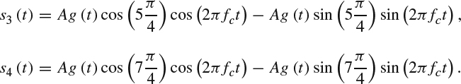
• M-ary phase shift keying (MPSK): in this modulation scheme, blocks of b bits are mapped into different phases. Since there are M = 2^b different blocks with b bits, the modulated signal is:

  

  where i = 1, 2, …, M, is the index assigned to each possible block of input bits, A is a constant to determine the transmit power and g(t) is a non-information-carrying signal used to shape the spectral signature of the modulated signal.

• Binary phase shift keying (BPSK): this is a very important particular case of MPSK, where b = 1. Therefore, with i = 1, 2, the two possible modulated signals are:

  

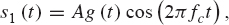
  mapped, for example, to an input bit equal to zero, and:

  

  mapped in the example to an input bit equal to one. Note how the two modulated signals differ by a phase of 180°.

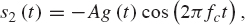
• Quaternary phase shift keying (QPSK): this is another important particular case of MPSK where b = 2. Therefore, with i = 1, 2, 3, 4, the four possible input blocks ‘00’, ‘01’, ‘10’, and ‘11’ are mapped to the modulated signals:

  

• Quadrature amplitude modulation (QAM): in this modulation scheme the group of input bits is mapped into modulated signals changing both in phase and amplitude. This means that a QAM signal is of the form:

  

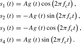
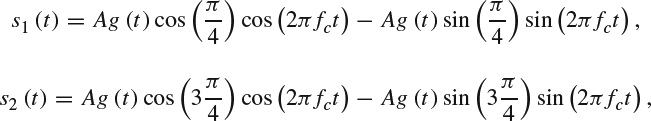
  One common case of QAM is 4QAM, where b = 2 and M = 4, for which the modulating signals are:

  

  

  Other common cases of QAM are 16QAM, where b = 4 and M = 16, and 32QAM, where b = 5 and M = 32.

6.2.2 The Wireless Channel

The communication of information over wireless links presents specially challenging problems due to the nature of the wireless channel itself, which introduce severe impairments to the transmitted signal. Understanding these impairments is of fundamental importance in understanding any wireless communications system. As such, we present in the rest of this section a summary of the main wireless channel characteristics.

The simplest of all impairments are those that add a random noise to the transmitted signal. One source for this type of random noise is interference. Additive white Gaussian noise (AWGN) is another very good and important example of this type of additive impairment. Modeling the AWGN as a channel results in the additive white Gaussian noise, where the relation between the output y(t) and the input signal x(t) is given by Figure 6.2,

where γ is the loss in power of the transmitted signal, x(t), and n(t) is noise. The additive noise n(t) is a random process where each sample, or realization, is modeled as a random variable with a Gaussian distribution. This noise term is generally used to model background noise in the channel as well as noise introduced at the receiver front end. Also, the AWGN is frequently assumed for simplicity to model some types of interference although, in general, these processes do not strictly follow a Gaussian distribution.

Other wireless channel impairments are classified as either “large-scale propagation effects” or “small-scale propagation effects”, where the “scale” in the class names refers to the relative change of distance between transmitter and receiver that is necessary to experience changes in effect magnitude.

Among the large-scale propagation effects, the path loss is an important effect that contributes to signal impairment by reducing the propagating signal power as it propagates further away from the transmitter to the receiver. The path loss, γ_dB, is measured as the value in decibels of the ratio between the received P_R and transmitted signal power P_T:

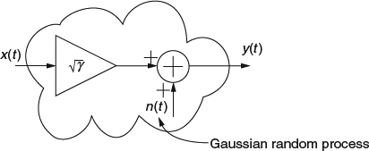
Figure 6.2 Additive white Gaussian noise (AWGN) channel model.

The value of the path loss is highly dependent on many factors related to the entire transmission setup. In general, the path loss is characterized by a function of the form:

where d is the distance between transmitter and receiver, v is the path loss exponent, c is a constant and d₀ is the distance to a power measurement reference point (sometimes embedded within the constant c). In many practical scenarios this expression is not an exact characterization of the path loss, but is still used as a sufficiently good and simple approximation. The constant c includes parameters related to the physical setup of the transmission such as signal wavelength, antenna heights, etc. The path loss exponent v characterizes the rate of decay of the signal power with the distance. If the path loss, measured in dB, is plotted as a function of the distance on a logarithmic scale, the function in (6.1) is a line with a slope − v. The path loss exponent takes values in the range of 2 to 6, with 2 being the best case scenario, which corresponds to signal propagation in free space. Typical values for the path loss exponent are 4 for an urban macro cell environment and 3 for an urban micro cell.

Equation (6.1) shows the relation between the path loss and the distance between the transmit and receive antennas, but it does not characterize all the large-scale propagation effects. In practice, the path losses of two receive antennas situated at the same distance from the transmit antenna are not the same. This is, in part, because different objects may be obstructing the transmitted signal as it travels to the receive antenna. Consequently, this type of impairment has been named shadow loss or shadow fading. Since the nature and location of the obstructions causing shadow loss cannot be known in advance and is inherently random, the path loss introduced by this effect is itself a random variable. Denoting by S the value of the shadow loss, this effect can be incorporated into (6.1) by writing:

Through experimental measurements it has been found that S when measured in dB can be characterized as a zero-mean Gaussian distributed random variable. Consequently, the shadow loss magnitude is a random variable that follows a log-normal distribution and its effect is frequently referred as log-normal fading.

As discussed earlier, large-scale propagation effects owe the name to the fact that their effects are noticeable over relatively long signal propagation distances. In contrast, for small-scale propagation effects, the effects are noticeable at distances in the order of the signal wavelength. These effects appear as a consequence of multiple copies of the signal arriving at the receiver after each has traveled through different paths. This is because radio signals do not usually arrive at the receiver following a direct line-of-sight propagation path but, instead, arrive after encountering random reflectors, scatterers and attenuators during propagation. Such a channel where a transmitted signal arrives at the receiver with multiple copies is known as a multipath channel. Several factors influence the behavior of a multipath channel. In addition to the already mentioned random presence of reflectors, scatterers and attenuators, the speed of the mobile terminal, the speed of surrounding objects and the transmission bandwidth of the signal, are other factors determining the behavior of the channel. Furthermore, the multipath channel is likely to change over time because of the presence of motion at the transmitter, at the receiver, or at the surrounding objects. The multiple copies of the transmitted signal arriving through a different propagation path will each have a different amplitude, phase and delay. The multiple signal copies are added at the receiver creating either constructive or destructive interference with each other. This results in a time varying received signal. Therefore, if denoting the transmitted signal by x(t) and the received signal by y(t), their relation can be written as:

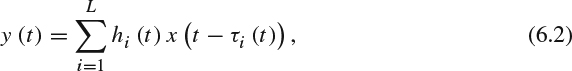
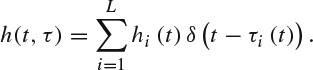
where h_i(t) is the attenuation of the ith path at time t, τ_i(t) is the corresponding path delay and L is the number of resolvable paths at the receiver. This relation implicitly assumes that the channel is linear, for which y(t) is equal to the convolution of x(t) and the channel impulse response as seen at time t to an impulse sent at time τ, h(t, τ). From (6.2), this impulse response can be written as:

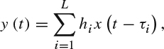
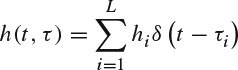
Furthermore, in cases when it is safe to assume that the channel does not change over time, there is no need to maintain the functional dependency on time, thus, the received signal can be simplified as:

and the channel impulse response as:

When studying the communication of digital information and sources it is convenient to abstract the whole communication system as a complete discrete-time system. The model obtained with this approach is called the discrete-time baseband-equivalent model of the channel, for which the input–output related with the mth discrete time instant can be written as:

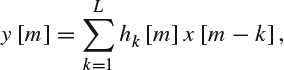
where h_k[m] are the channel coefficients from the discrete-time channel impulse response. In this relation it is implicit that there is a sampling operation at the receiver and that all signals are considered as in the baseband equivalent model. The conversion to a discrete-time model combines all the paths with arrival time within one sampling period into a single channel response coefficient h_k[m] Also, note that the discrete-time channel model is just a time-varying FIR digital filter. In fact, it is quite common to call the channel model based on the impulse response in the same way as FIR filters are called, as the tapped-delay model. Since the nature of each path, its length and the presence of reflectors, scatterers and attenuators are all random, the channel coefficients h_k[m] of the discrete-time channel model are random processes. If, in addition, it can be assumed that the channel model is not changing over time, then the channel coefficients h[m] of a time-invariant discrete-time channel model are random variables (and note that the redundant time index needs not be specified).

In the discrete-time impulse response model for a wireless channel, each coefficient indicates the attenuation and change of phase for the collection of signals arriving through multiple paths within the same sampling interval. The attenuation of each coefficient is directly related with the power attenuation for each path. The function determined by the average power associated with each path (with a path actually being a collection of paths arriving within the same sample interval) is called the power delay profile of the multipath channel. As an illustrative example, Figure 6.3 shows the power delay profile for a typical multipath wireless channel. The example reproduces the wireless channel models specified by the International Telecommunications Union in its standard ITU-R M.1225, [8].

In order to characterize the channel, several parameters are associated with the impulse response but calculated from the power delay profile or its spectral response (Fourier transform of the power delay profile). These parameters allow the classification of different multipath channels based on how they affect a transmitted signal. The first of these parameters is the channel delay spread. The channel delay spread is defined as the time difference between the arrival of the first measured path and the last (there are a few alternative, conceptually similar, definitions but their discussion is irrelevant to this book). Note that, in principle, there may be several signals arriving through very attenuated paths, which may not be measured due to the sensitivity of the receiver. This means that the concept of delay spread is tied to the sensitivity of the receiver.

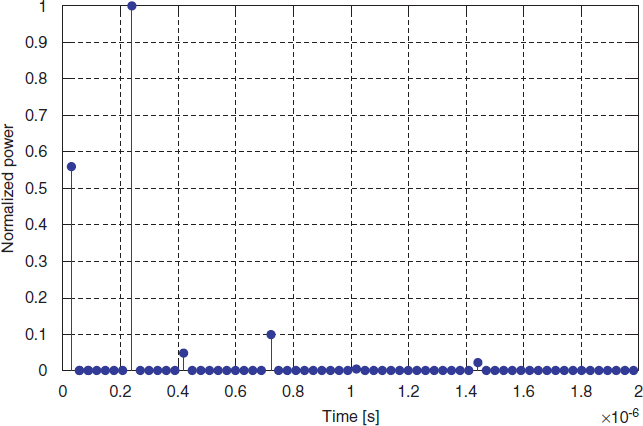
Figure 6.3 The power delay profile for a typical multipath channel. The figure shows the power from each path normalized to the maximum path power.

A second parameter is the coherence bandwidth, which is the range of frequencies over which the amplitude of two spectral components of the channel response are correlated (similar to the power delay profile, there are other similar definitions, which will not be discussed here). The coherence bandwidth provides a measurement of the range of frequencies over which the channel shows a flat frequency response, in the sense that all the spectral components have approximately the same amplitude and a linear change of phase. This means that if the transmitted information-carrying signal has a bandwidth that is larger than the channel coherence bandwidth, then different spectral components of the signal will be affected by different attenuations, resulting in a distortion for the spectrum and the signal itself. In this case, the channel is said to be a frequency-selective channel or a broadband channel. In contrast, when the bandwidth of the information-carrying signal is less than the channel coherence bandwidth, then all the spectral components of the signal will be affected by the same attenuation and by a linear change of phase. In this case, the received signal (i.e., that at the output of the channel) will have practically the same spectrum as the transmitted signal and thus will suffer from little distortion. This type of channel is said to be a flat-fading channel or a narrowband channel.

Note that while we just described different types of channels, whether a particular channel will appear as being of one type or another (i.e., flat-fading or frequency-selective) does not only depend on the channel, but it also depends on the characteristics of the signal at the input of the channel and how they relate with the characteristics of the channel. To better understand this, Figure 6.4 shows a section of the spectral response of the channel with the power delay profile shown in Figure 6.3. In principle, by looking at Figure 6.4 only, it is not possible to tell whether the channel is a flat fading or a frequency-selective channel. Indeed, the channel frequency response may be seen as roughly flat by a signal with bandwidth equal to a few tens of kHz, but it would be seen as frequency-selective by a signal with a larger bandwidth. To see this, consider that the transmitted signal is a single raised cosine pulse with roll-off factor 0.25 and symbol period 0.05 μs. The pulse is shown on the left of Figure 6.5. The corresponding spectrum can be seen on the right of Figure 6.4. The bandwidth for the transmitted pulse is approximately 2 MHz. As shown in Figure 6.6, the large bandwidth of the transmitted pulse makes the channel behave as a frequency-selective channel, resulting in a distorted transmitted pulse spectrum at the output of the channel.

It is important to understand the distorting effects of a frequency-selective channel in the time domain. Here, the transmitted pulse with a bandwidth that is larger than the channel coherence bandwidth translates into a channel delay spread that is much larger than the duration of the pulse. In this case, and since the channel affects a transmitted pulse by performing a convolution, at the output of the channel there is going to be one delayed and attenuated replica of the transmitted pulse for each of the discernible channel paths. Because of this, the pulse at the output of the channel will see its duration extended to that of the delay spread and its shape severely distorted. This is illustrated in Figure 6.7 where, at the top, it shows the pulse from Figure 6.5 after being transmitted through the channel in Figure 6.3. The figure shows all the pulses arriving through each of the channel paths. The resulting pulse is equal to the addition of the pulses from each of the paths.

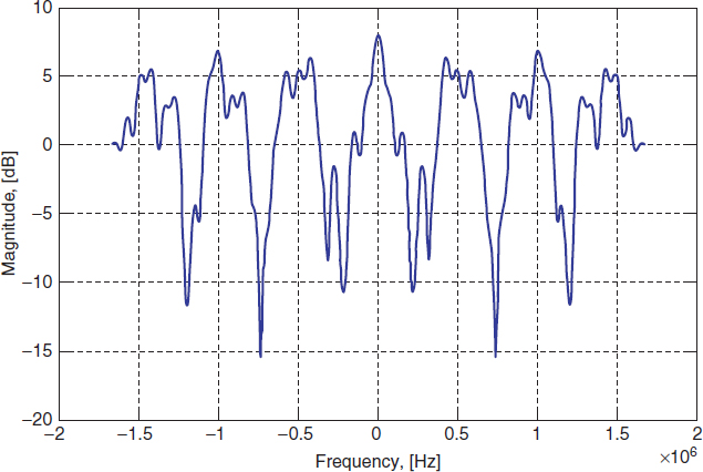
Figure 6.4 Section of the magnitude frequency response for the channel with the power delay profile in Figure 6.3.

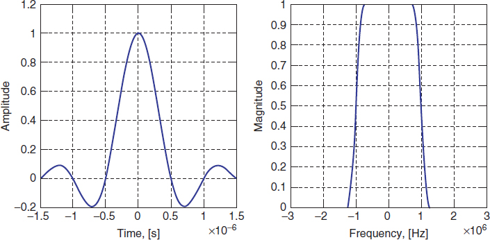
Figure 6.5 The short duration raised cosine pulse sent over the channel in Figure 6.3 – on the left, the time domain signal, on the right, its corresponding magnitude spectrum.

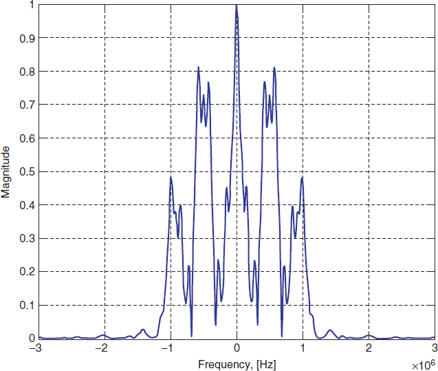
Figure 6.6 The spectrum of the raised cosine pulse in Figure 6.5 after being transmitted through the channel in Figure 6.3.

Figure 6.8 concludes the illustration of a frequency-selective channel by showing the input and output pulses in both the time and frequency domains. It is important to note here how the frequency-selective channel is associated with a large delay spread. The fact that a time domain phenomenon such as instances of a signal arriving with different delays, translates into a frequency domain effect, such as frequency selectivity, can be understood in the following way. When the signals with different delays from the multipath get superimposed at the receive antenna, the different delay translates into different phases. Depending on the phase difference between the spectral components, their superposition may result into destructive or constructive interference. Even more, because the relation between phase and path delay for each spectral component of the arriving signal varies with the frequency of the spectral component, the signal will undergo destructive or constructive interference of different magnitude for each spectral component, resulting in the frequency response of the channel not appearing as a constant amplitude. The extension of the pulse duration has important effects when sending several pulses in succession (as would usually happen when transmitting a bit stream) because the pulses at the output of the channel will overlap with other pulses sent earlier or later. This overlap of transmitted symbols is called inter-symbol interference (ISI).

Comparing the effects of frequency-selective channel versus a non-frequency-selective channel, Figures 6.9 through 6.11 shows the time and frequency domains input and output signals to the channel in Figures 6.3 and 6.4 when the input pulse have a transmission period long enough for the channel to behave as non-frequency-selective. In this case, the input pulse has a bandwidth of approximately 2 kHz, for which the frequency response of the channel appears roughly flat. At the same time, the duration of the input pulse is several times longer than the channel delay spread, which results in little difference relative to the pulse duration in the time each pulse takes to arrive through a different path. In other words, with the longer duration of the pulse, the delays associated with different channel paths can be practically neglected and there is no ISI. Consequently, the transmitted pulse suffers little alterations in both time and frequency domains. While a longer duration pulse avoids the challenges associated with a frequency-selective channel, it also limits the data rate at which information can be sent over the channel.

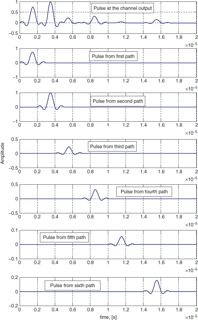
Figure 6.7 The raised cosine pulse in Figure 6.5 after being transmitted through the channel in Figure 6.3 (top). The pulse is the result of adding all the pulses received from each of the channel's paths (in plots below the top one).

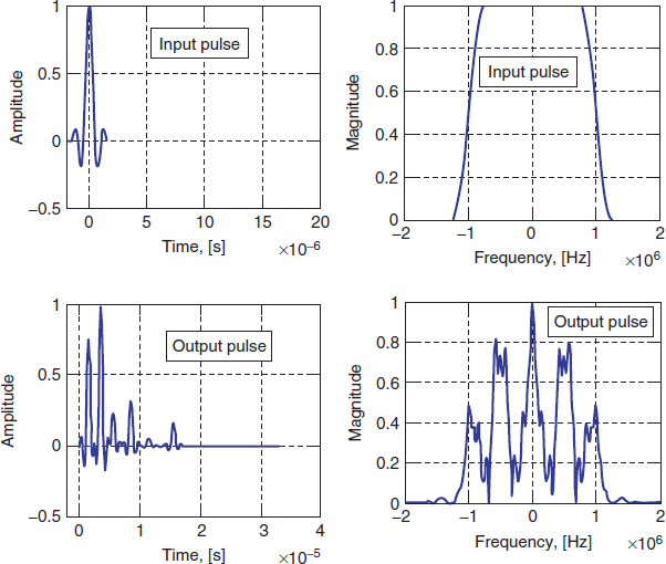
Figure 6.8 Summary of the effects of a frequency-selective channel showing the raised cosine pulse in Figure 6.5 at the input and at the output of the channel, both in time and frequency domain.

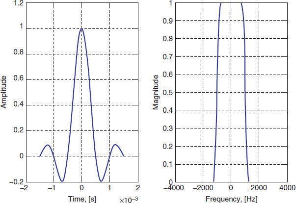
Figure 6.9 The long duration raised cosine pulse sent over the channel in Figure 6.3 – on the left, the time domain signal, on the right, its corresponding magnitude spectrum.

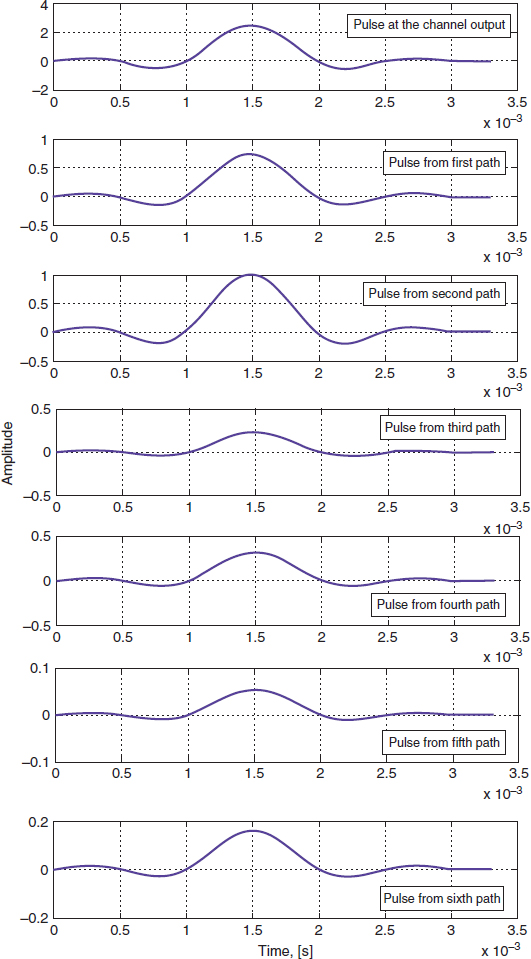
Figure 6.10 The raised cosine pulse in Figure 6.9 after being transmitted through the channel in Figure 6.3 (top). The pulse is the result of adding all the pulses received from each of the channel's paths (in plots below the top one).

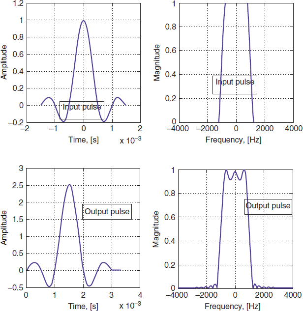
Figure 6.11 Summary of the effects of a non-frequency-selective channel showing the raised cosine pulse in Figure 6.9 at the input and at the output of the channel, both in time and frequency domain.

As mentioned earlier in this section, the motions of the transmitter, the receiver or the signal reflectors along the signal propagation path creates a change in the channel impulse response over time. As such, there are parameters that describe the time-varying characteristics of the wireless channel. The most notable effect introduced by mobility is a shift in frequency due to Doppler shift. To characterize the channel in terms of Doppler shift, the parameters usually considered are the channel coherence time and the Doppler spread.

As a channel changes over time, the coefficients of the impulse response, and thus the impulse response itself, become a random process, with each realization at different time instants being a random variable. These random variables may or may not be correlated. The channel coherence time is the time difference that makes the correlation between two realizations of the channel impulse response be approximately zero. The Fourier transform of the correlation function between the realizations of a channel coefficient is known as the channel Doppler power spectrum, or simply the Doppler spectrum. The Doppler spectrum characterizes in a statistical sense how the channel affects an input signal and widens its spectrum due to Doppler shift. This means that if the transmitter injects into the channel a single-tone sinusoidal signal with frequency, f_c, the Doppler spectrum will show frequency components in the range f_c − f_d to f_c + f_d, where f_d is the channel's Doppler shift.

The second parameter usually used to characterize the effects of the channel time variations is the Doppler spread. This is defined as the range of frequencies over which the Doppler power spectrum is nonzero. It can be shown that the Doppler spread is the inverse of the channel coherence time and as such, provides information on how fast the channel changes over time. Similarly to the discussion on frequency selectivity of a channel – a characteristic that depended both on the channel and the input signal – the notion on how fast the channel is changing over time depends also on the input signal. If the channel coherence time is larger than the transmitted signal symbol period, or equivalently, if the Doppler spread is smaller than the signal bandwidth, the channel will be changing over a period of time longer than the input symbol duration. In this case, the channel is said to have slow fading. If the reverse is true, the channel is said to have fast fading.

We now turn our attention towards the random nature of the channel coefficients and the important related question of what are their statistical properties and what kind of mathematical model can characterize this behavior. There are several models to statistically characterize the channel coefficients; some are analytical, obtained from proposing a simplified representative model, and other models are empirical, having been derived by matching functions to the results of field measurements. One of the most common analytical models for the random channel coefficients is based on an environment known as the “Uniform Scattering Environment”. Since this model was introduced by R. H. Clarke and later developed by W. C. Jakes, the model is also known as Clarke's model or Jakes' model. The key assumption in this model is that there is no dominant line-of-sight (LOS) propagation and that a waveform arrives at a receiver through a multipath channel resulting from a very large number of scatterers along the signal path. Furthermore, the scatterers are assumed to be randomly located on a circle centered on the receiver (see Figure 6.12) and that they create a very large number of paths arriving from the scatterers at an angle that is uniformly distributed between 0 and 2π. Furthermore, it is assumed that all the received signals arrive with the same amplitude. This is a reasonable assumption because, given the geometry of the uniform scattering environment, in the absence of a direct LOS path, each signal arriving at the receiver would experience similar attenuations.

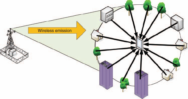
Figure 6.12 The uniform scattering environment.

The theoretical study of the uniform scattering model results in the conclusion that each channel coefficient can be modeled as a circularly symmetric complex Gaussian random variable with zero mean; that is, as a random variable made of two quadrature components, with each component being a zero mean Gaussian random variable with the same variance as the other component σ². From this conclusion, it is further possible to derive the probability density function for the magnitude and phase of the complex-valued channel coefficients (i.e., by writing the coefficients in the form h = re^jθ). By following straightforward random variables transformation theory, it follows that the magnitude of the channel coefficients is a random variable with a Rayleigh distribution with probability density function (pdf):

and the phase is a random variable with a uniform distribution in the range [0, 2π] and with pdf: f_θ(x) = 1/(2π). Because of the probability distribution for the channel coefficient magnitude, this model is also called the Rayleigh fading model. It is also of interest to calculate the probability density function of the random variable |h|², the channel coefficient power gain. By applying again random variables transformation theory, it follows that |h|² is an exponential random variable with probability density function:

The Rayleigh fading model is not the only model for the channel coefficients. In fact, in deriving the Rayleigh fading for the uniform scattering environment it was assumed that all the received signals arrive with the same amplitude due to the absence of a direct LOS path and the symmetric geometry of the environment. When there is one LOS path that is received with a dominant power, the assumptions corresponding to the Rayleigh fading model do not hold any more. With the LOS path, the two Cartesian components of the complex-valued channel coefficient are still a Gaussian random variables but now one has a nonzero mean A, which is the peak amplitude of the signal from the line-of-sight path. In this case, it can be shown that the magnitude of the channel coefficient is a Rician-distributed random variable with a probability density function:

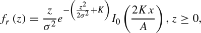
where K is a parameter of the Ricean distribution defined as:

and I₀(x) is the modified Bessel function of the first kind and zero order, defined as:

Note that in the Rician distribution when K = 0, the Rician probability density function becomes equal to the Rayleigh probability density function. This is consistent with the fact that K = 0 implies that A = 0, that is, there is no LOS path.

As mentioned earlier in this section, another approach to modeling the wireless channel follows an empirical procedure where samples of a practical channel are measured on the field and then the statistics of these samples are matched to a mathematical model. For this it is useful to have a probability density function that can be easily matched to the different possible data sample sets. This function is provided by the Nakagami fading distribution, which has a probability density function given by:

where Γ(z) is the Gamma function:

and m is a parameter used to adjust the pdf of the Nakagami distribution to the data samples. For example, if m = 1, then the Nakagami distribution becomes equal to the Rayleigh distribution. One advantage of the Nakagami distribution is that it matches empirical data better than other distributions. In fact, the Nakagami distribution was originally proposed for this very reason.

To summarize the discussion on different random variable distributions for modeling channel fading, Figure 6.13 shows the pdfs presented in this section.

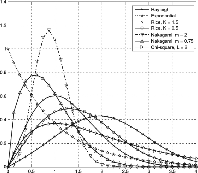
Figure 6.13 Different probability density functions used to model random fading.

6.2.3 Adaptive Modulation and Coding

As should be clear from the discussion so far, the principal characteristic for wireless communications is the need to cope with severe impairments of the channel. For a modulated signal, these impairments will distort the signal to an extent that may result in the receiver misinterpreting the signal for another of the possible modulated signals. When this happens, the demodulator at the receiver will output an erred decision on the transmitted information. The likelihood of this error happening will, of course, depend on the quality of the channel, with worse channels leading to errors with a higher probability. At the same time, and while there are many possible receiver technologies, as a general rule, modulation techniques that achieve a higher bit rate by packing more bits per symbol are also more susceptible to errors. Figure 6.14 illustrates this point by showing the bit error rate as a function of AWGN channel SNR for three MPSK schemes. In the figure it can be seen that if, for example, the channel SNR is 8 dB, then transmission using 16-PSK will have a bit error rate in the order of 10⁻², transmission using 8-PSK will have a bit error rate approximately ten times less, and transmission using BPSK will have a bit error rate approximately equal to 10⁻⁴.

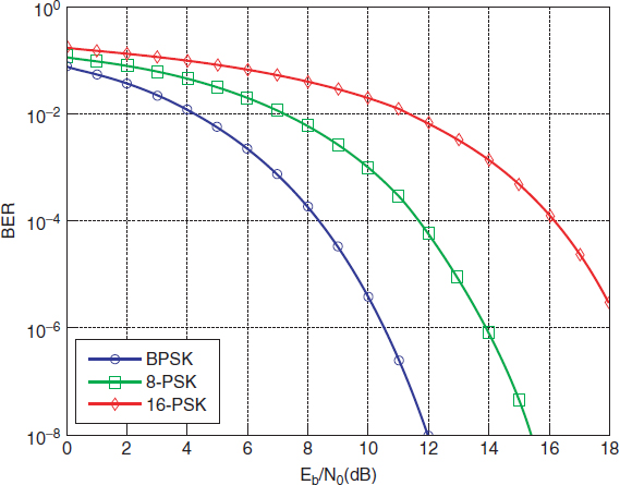
Figure 6.14 Bit error rate as a function of channel signal-to-noise ratio for three cases of MPSK modulation (M = 2, M = 8 and M = 16).

Figure 6.14 can also be interpreted with a different approach. Assume, as is usually the case, that the traffic being transmitted requires a minimum bit error rate performance during communication. For the sake of this presentation, let us suppose that the requirement is that bit error rate cannot exceed 10⁻⁴. In this case, then, Figure 6.14 shows that if the channel SNR is below 8dB, it will not be possible to meet the service requirement for maximum BER, regardless of the modulation scheme being used. If the channel SNR is between 8 and 12 dB, the transmission will have to use BPSK because it is the only modulation scheme with BER less than 10⁻⁴. If the channel SNR is between 12 and 16 dB, there is a choice between BPSK and 8-PSK for transmission because both modulation schemes have BER less than 10⁻⁴. Finally, for channel SNRs above 16 dB it would be possible to choose any of the three modulation schemes in Figure 6.14.

When it is possible to choose between different modulation schemes, it is better to choose the one that results in higher transmit bit rate. For the case of Figure 6.14, BPSK sends one bit per modulation symbol, 8-PSK sends three and 16-PSK sends four. Therefore, 16-PSK shows four times the bit rate of BPSK and 8-PSK three times the bit rate of BPSK. Consequently, from the performance shown in Figure 6.14, if the channel SNR is more than 16 dB, the modulation used during transmission would be 16-PSK; if the channel SNR is 12 and 16 dB, the transmission would use 8-PSK; and if channel SNR is between 8 and 12 dB, the transmission would use BPSK. If the channel SNR is less than 8 dB, it would not be possible to meet the maximum BER requirement for modulation choice. Of course, it is usually the case that some type of forward error control (FEC) technique is used during transmission. With FEC, adding extra redundant bits results in a stronger protection against channel errors, allowing meeting the maximum BER requirement at lower channel SNR. At the same time, when using FEC, the extra redundant bits reduce the number of information bits that can be transmitted per unit time when the transmit bit rate is fixed. In other words, the more error protection (equivalently, the more redundant bits) that is added to the transmitted bit stream, the lower the channel SNR that can be used for transmission satisfying BER constraints but, also, the less information bits are transmitted per unit time.

The above discussion highlights that there are two interlinked tradeoffs determining the choice of transmission parameters. One tradeoff is the transmit bit rate versus the channel SNR. The second tradeoff is the amount of FEC redundancy for error protection in a given channel SNR versus the effective transmitted information bit rate. The modulation scheme and the level of FEC redundancy can be chosen at design time after carefully considering these tradeoffs. Nevertheless, modern communication systems allow for a dynamic adaptation of these transmit parameters based on the channel conditions (e.g., channel SNR). This technique is called adaptive modulation and coding (AMC). In AMC, the transmitter uses estimates of the channel state to choose a modulation scheme and a level of FEC redundancy that maximizes the transmitted information bit rate for a given channel SNR.