Chapter 12. Advanced Query Techniques

IN THIS CHAPTER

• Why This Chapter Is Important
• Using Action Queries
• Viewing Special Query Properties
• Optimizing Queries
• Using Crosstab Queries
• Establishing Outer Joins
• Establishing Self-Joins
• Understanding SQL
• Building Union Queries
• Using Pass-Through Queries
• Examining the Propagation of Nulls and Query Results
• Running Subqueries
• Using SQL to Update Data
• Using SQL for Data Definition
• Using the Result of a Function as the Criteria for a Query
• Passing Parameter Query Values from a Form
• Understanding Jet 4.0 ANSI-92 Extensions
• Practical Examples: Applying These Techniques in Your Application

Why This Chapter Is Important

You learned the basics of query design in Chapter 4, “What Every Developer Needs to Know About Query Basics,” but Access has a wealth of query capabilities. In addition to the relatively simple Select queries covered in Chapter 4, you can create crosstab queries, union queries, self-join queries, and many other complex selection queries. You can also easily build Access queries that modify information, rather than retrieve it. This chapter covers these topics and the more advanced aspects of query design.

Using Action Queries

With action queries, you can easily modify data without writing code. In fact, using action queries is often a more efficient method than using code. Four types of action queries are available: update, delete, append, and make table. You use update queries to modify data in a table, delete queries to remove records from a table, append queries to add records to an existing table, and make table queries to create an entirely new table. Each type of query and its appropriate uses are explained in the following sections.

Update Queries

You use update queries to modify all records or any records meeting specific criteria. You can use an update query to modify the data in one field or several fields (or even tables) at one time (for example, a query that increases the salary of everyone in California by 10%). As mentioned, using update queries is usually more efficient than performing the same task with Visual Basic for Applications (VBA) code, so update queries are considered a respectable way to modify table data.

To build an update query, follow these steps:

1. Click the Query Design tool in the Other group on the Create tab. The Show Table dialog box appears.
2. In the Show Table dialog box, select the tables or queries that will participate in the update query and click Add. Click Close when you’re ready to continue.
3. Click Update in the Query Type group on the Design tab.
4. Add fields to the query that will either be used for criteria or be updated as a result of the query. In Figure 12.1, StateProvince has been added to the query grid because it will be used as a criterion for the update. DefaultRate has been included because it’s the field that’s being updated.

   Figure 12.1. An update query that increases the DefaultRate for all clients in California.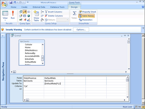

   

5. Add any further criteria, if you want. In Figure 12.1, the criterion for StateProvince has been set to CA.
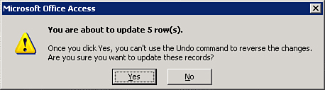
6. Add the appropriate Update expression. In Figure 12.1, the DefaultRate is being increased by 10%.
7. Click Run on the ribbon. The message box shown in Figure 12.2 appears. Click Yes to continue. The Access Database Engine updates all records meeting the selected criteria.

Figure 12.2. The confirmation message you see when running an update query.

You should name Access update queries with the prefix qupd. To adhere to standard naming conventions, you should give each type of action query a prefix indicating what type of query it is. Table 12.1 lists all the proper prefixes for action queries.

Table 12.1. Naming Prefixes for Action Queries

All Access queries are stored as Structured Query Language (SQL) statements. (Access SQL is discussed later in this chapter in the “Understanding SQL” section.) You can display the SQL for a query by selecting SQL view from the View drop-down on the Design tab. The SQL behind an Access update query looks like this:

Delete Queries

Rather than simply modify table data, delete queries permanently remove from a table any records meeting specific criteria; they’re often used to remove old records. You might want to delete all orders from the previous year, for example.

To build a delete query, follow these steps:

1. While in a query’s Design view, select Delete from the Query Type group on the Design tab.
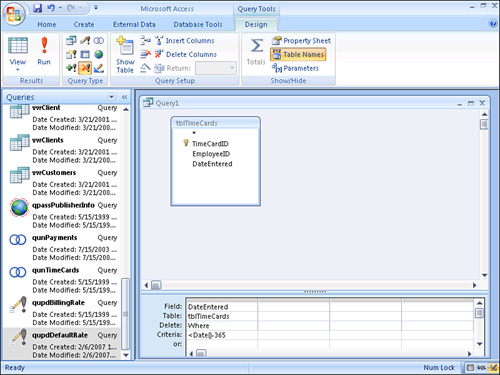
2. Add the criteria you want to the query grid. The query shown in Figure 12.3 deletes all time cards more than 365 days old.

   Figure 12.3. A delete query used to delete all time cards entered more than a year ago.

   

3. Click Run on the ribbon. The message box shown in Figure 12.4 appears.

   Figure 12.4. The delete query confirmation message box.

   

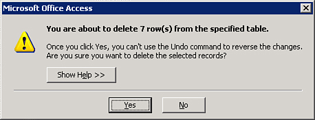
4. Click Yes to permanently remove the records from the table.

The SQL behind a delete query looks like this:

Append Queries

With append queries, you can add records to an existing table. This is often done during an archive process. First, you append the records to be archived to the history table by using an append query. Next, you remove them from the master table by using a delete query.

To build an append query, follow these steps:

1. While in Design view of a query, select Append from the Query Type group on the Design tab. The dialog box shown in Figure 12.5 appears.

   Figure 12.5. Identifying the table to which data will be appended and the database containing that table.

   

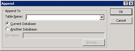
2. Select the table to which you want the data appended.
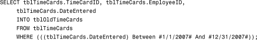
3. Drag all the fields whose data you want included in the second table to the query grid. If the field names in the two tables match, Access automatically matches the field names in the source table to the corresponding field names in the destination table (see Figure 12.6). If the field names in the two tables don’t match, you need to explicitly designate which fields in the source table match which fields in the destination table.

   Figure 12.6. An append query that appends the EmployeeID and DateEntered of all employees entered in the year 2007 to another table.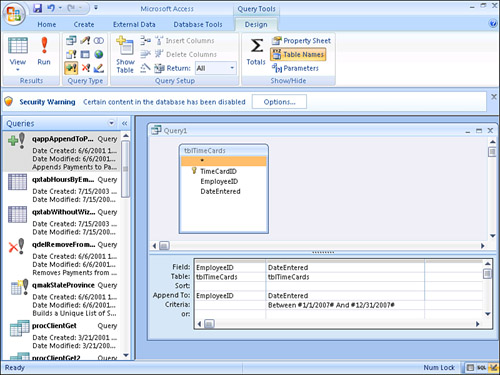

   

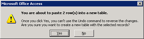
4. Enter any criteria in the query grid. Notice in Figure 12.6 that all records with a DateEntered in 2007 are appended to the destination table.
5. To run the query, click Run on the ribbon. The message box shown in Figure 12.7 appears.

   Figure 12.7. The append query confirmation message box.

   

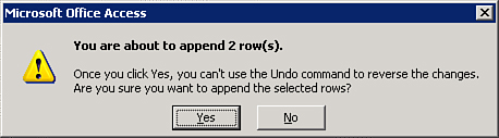
6. Click Yes to finish the process.

The SQL behind an append query looks like this:

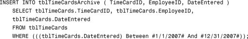
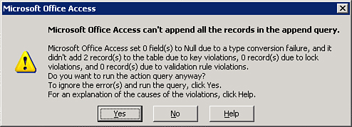
Append queries don’t allow you to introduce any primary key violations. If you’re appending any records that duplicate a primary key value, the message box shown in Figure 12.8 appears. If you go ahead with the append process, only those records without primary key violations are appended to the destination table.

Figure 12.8. The warning message you see when an append query and conversion, primary key, lock, or validation rule violation occurs.

Make Table Queries

An append query adds records to an existing table, but a make table query creates a new table, which is often a temporary table used for intermediary processing. You will often create a temporary table to freeze data while a user runs a report. By building temporary tables and running the report from those tables, you make sure users can’t modify the data underlying the report during the reporting process. Another common use of a make table query is to supply a subset of fields or records to a user.

To build a make table query, follow these steps:

1. While in the query’s Design view, select Make Table from the Query Type group on the Design tab. The dialog box shown in Figure 12.9 appears.

   Figure 12.9. Enter a name for the new table and select which database to place it in.

   

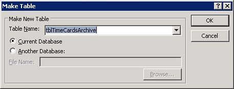
2. Enter the name of the new table and click OK.
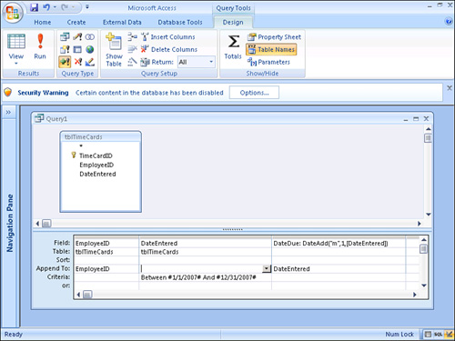
3. Move all the fields you want included in the new table to the query grid. The result of an expression is often included in the new table (see Figure 12.10).

   Figure 12.10. Add an expression to a make table query.

   

4. Add the criteria you want to the query grid.
5. Click Run on the ribbon to run the query. The message shown in Figure 12.11 appears.

   Figure 12.11. The make table query confirmation message box.

   

6. Click Yes to finish the process.

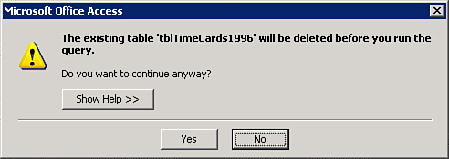
If you try to run the same make table query more than one time, the table with the same name as the table you’re creating is permanently deleted (see the warning message in Figure 12.12).

Figure 12.12. The make table query warning message displayed when a table already exists with the same name as the table to be created.

The SQL for a make table query looks like this:

Using Action Queries Versus Processing Records with Code

As mentioned previously, action queries can be far more efficient than VBA code. Look at this example:

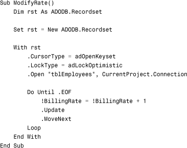
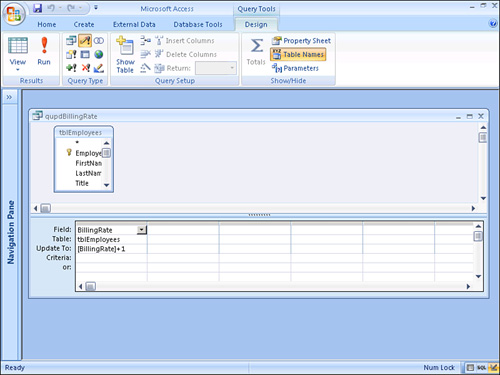
This subroutine uses ActiveX Data Objects (ADO) code to loop through tblEmployees. It increases the billing rate by 1. Compare the ModifyRate subroutine to the following code:

As you can see, the RunActionQuery subroutine is much easier to code. The qupdBillingRate query, shown in Figure 12.13, performs the same tasks as the ModifyRate subroutine. In most cases, the action query runs more efficiently.

Figure 12.13. The qupdBillingRate query increments the BillingRate by 1.

Viewing Special Query Properties

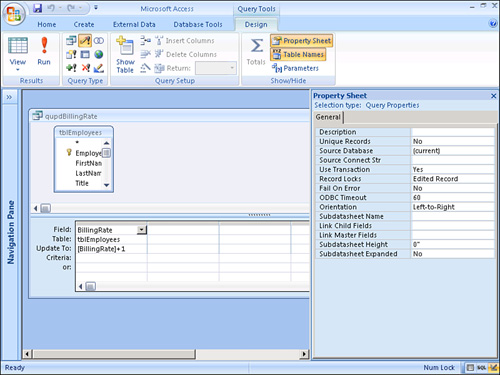
Access 2007 queries have several properties that can dramatically change their behavior. To look up a query’s properties, right-click on a blank area in the top half of the Query window and select Properties to open the Property Sheet (see Figure 12.14). Chapter 4 discusses many of these properties. The following sections cover the Unique Values, Unique Records, and Top Values properties.

Figure 12.14. Viewing the general properties for a query.

Unique Values Property

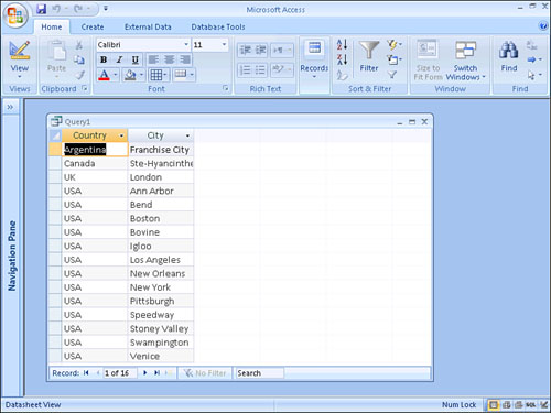
When set to Yes, the Unique Values property causes the query output to contain no duplicates for the combination of fields you include in it. Figure 12.15, for example, shows a query that includes the Country and City fields from tblClients. The Unique Values property in this example is set to No, its default value. Notice that many combinations of countries and cities appear more than once. This happens whenever more than one client is found in a particular country and city. Compare this with Figure 12.16, in which the Unique Values property is set to Yes. Each combination of country and city appears only once.

Figure 12.15. A query with the Unique Values property set to No.

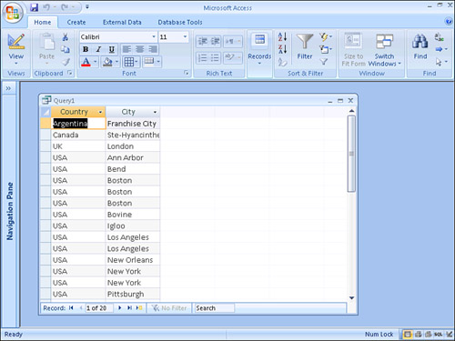
Figure 12.16. A query with the Unique Values property set to Yes.

Unique Records Property

In Access 2000 and later, the default value for the Unique Records property is No. Setting it to Yes causes the DISTINCTROW statement to be included in the SQL statement underlying the query. When set to Yes, the Unique Records property denotes that the Access Database Engine includes only unique rows in the recordset underlying the query in the query result—and not just unique rows based on the fields in the query result. The Unique Records property applies only to multitable queries; the Access Database Engine ignores it for queries that include only one table.

Top Values Property

The Top Values property enables you to specify a certain percentage or a specific number of records that the user wants to view in the query result. For example, you can build a query that outputs the country/city combinations with the top 10 sales amounts. You can also build a query that shows the country/city combinations whose sales rank in the top 50%. You can specify the Top Values property in a few different ways. Here are two examples:

• Click the Top Values combo box on the ribbon and choose from the predefined list of choices (this combo box is not available for certain field types).
• Type a number or a number with a percent sign directly into the Top Values property in the Query Properties window, or select one of the predefined entries from the drop-down list for the property.

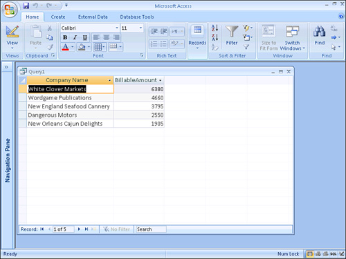
Figure 12.17 illustrates the design of a query showing the companies with the top 25% of sales. This Total query summarizes the result of the BillableHours multiplied by the BillingRate for each company. Notice that the Top Values property is set to 25%. The output of the query is sorted in descending order by the result of the BillableAmount calculation (see Figure 12.18). If the SaleAmount field were sorted in ascending order, the bottom 10% of the sales amount would be displayed in the query result. Remember that the field(s) you want to use to determine the top values must appear as the left-most field(s) in the query’s sort order.

Figure 12.17. A Total query that retrieves the top 25% of the billable amounts.

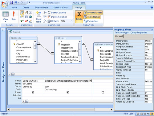
Figure 12.18. The result of a Total query showing the top 25% of the billable amounts.

Optimizing Queries

The Access Database Engine includes an Optimizer that looks at how long it takes to perform each task needed to produce the required query results. It then produces a plan for the shortest path to get the results that you want. This plan is based on several statistics:

• The amount of data in each table included in the query
• How many data pages are in each table
• The location of each table included in the query
• What indexes are available in each table
• Which indexes are unique

Understanding the Query Compilation Process

The statistics just listed are updated whenever the query is compiled. For a query to be compiled, it must be flagged as needing to be compiled. The flag can be any of the following occurrences:

• Changes are saved to the query.
• Changes are saved to any tables underlying a query.
• The database is compacted.

After the Access Database Engine flags a query as needing to be compiled, it isn’t compiled until the next time the query is run. During compiling, which takes 1–4 seconds, all statistics are updated, and a new optimization or Query Plan is produced.

Analyzing a Query’s Performance

When you’re analyzing the time it takes for a particular query to run, it’s important to time two tasks:

• How long it takes for the first screen of data to display
• How long it takes to get the last record in the query result

The first measurement is fairly obvious; it measures the amount of time it takes from the moment the Run button is clicked on the ribbon until the first screen of data is displayed. The second measurement is a little less obvious; it involves waiting until the N value in Record 1 of N displays at the bottom of the query result. The two measurements might be the same, if the query returns only a small number of records. The Access Database Engine decides whether it’s more efficient to run the query and then display the query results, or to display partial query results while the query continues to run in the background.

Steps You Can Take to Improve a Query’s Performance

You can take many steps to improve a query’s performance. They include, but aren’t limited to, the following techniques:

• Index fields on both sides of a join. If you establish a permanent relationship between two tables, the foreign key index is automatically created for you.
• Add to the query grid only the fields you actually need in the query results. If a field is required for criteria, but it doesn’t need to appear in the query result, clear the Show check box on the query grid.
• Add indexes for any fields that you are using in the sort order of the query result.
• Always index on fields used in the criteria of the query.
• Compact the database often. During compacting, Access tries to reorganize a table’s records so that they reside in adjacent database pages, ordered by the table’s primary key. The Access Database Engine rebuilds the query plans, based on the current amount of data. These side effects of the compacting process improve performance when the Access Database Engine is scanning the table during a query.
• When running a multitable query, test to see whether the query runs faster with the criteria placed on the “one” side or the “many” side of the join.
• Avoid adding criteria to calculated or nonindexed fields.
• Select the smallest field types possible for each field. For example, create a Long Integer CustID field instead of specifying the CompanyName field as the primary key for the table.
• Avoid calculated fields in nested queries. It’s always preferable to add calculations to the higher-level queries.
• Instead of including all expressions in the query, consider placing some expressions in the control source of form and report controls. If you do this, the expression will need to be repeated and maintained on each form and report.
• Use make table queries to build tables out of query results based on tables that rarely change. In a State table, for example, instead of displaying a unique list of states based on all the states currently included in the Customer table, build a separate State table and use that in your queries.
• When using Like in the query criteria, try to place the asterisk at the end of the character string rather than at the beginning. When you place the asterisk at the end of a string, as in Like Th*, an index can be used to improve query performance. If you place the asterisk at the beginning of a string, as in Like *Sr, the Access Database Engine cannot use any indexes.
• Use Count(*) rather than Count([fieldname]) when counting how many records meet a particular set of criteria. Count(*) simply tallies up the total number of records, but Count([fieldname]) actually checks to see whether the value is Null, which would exclude the record from the total computation. Furthermore, as mentioned in the next section on Rushmore technology, the Count(*) function is highly optimized by Rushmore.
• Use Group By as little as possible. When possible, use First instead. For example, if you’re totaling sales information by order date and order number, you can use First for the order date and group by order number. The reason is that all records for a given order number automatically occur on the same order date.
• Use Rushmore technology to speed query performance whenever possible. Rushmore technology—a data-access technology “borrowed” from Microsoft’s FoxPro PC database engine—improves the performance of certain queries. The following section discusses Rushmore technology.

One of the most important lessons to learn about the tips listed here is that you shouldn’t follow them blindly. Query optimization is an art, not a science. What helps in some situations might actually do harm in others, so it’s important to perform benchmarks with your actual system and data.

Rushmore Technology

Rushmore is a data-access technology that can help improve processing queries. You can use Rushmore technology only when you include certain types of expressions in the query criteria. It won’t automatically speed up all your queries. You must construct a query in a certain way for the query to benefit from Rushmore.

Rushmore can optimize a query with an expression and a comparison operator as the criteria for an Indexed field. The comparison operator must be <, >, =, <=, >=, <>, Between, Like, or In.

The expression can be any valid expression, including constants, functions, and fields from other tables. Here are some examples of expressions that Rushmore can optimize:

[Age] > 50
[OrderDate] Between #1/1/2007# And #12/31/2007#
[State] = "CA"

Rushmore can also optimize queries that include complex expressions combining the And and Or operators. If Rushmore can optimize both expressions, the query will be fully optimized. However, if Rushmore can optimize only one expression and you combine the expressions with an And, the query will be partially optimized. If Rushmore can fully optimize only one expression and you combine the expressions with an Or, the query won’t be optimized.

Important Notes About Rushmore

You should remember a few important concepts about Rushmore:

• Queries containing the Not operator can’t be optimized.
• The Count(*) function is highly optimized by Rushmore.
• Descending indexes cannot be used by Rushmore unless the expression is =.
• Queries on Open Database Connectivity (ODBC) data sources can’t use Rushmore.
• Rushmore can use multi-field indexes only when the criteria are in the order of the index. For example, if an index exists for the LastName field in combination with the FirstName field, the index can be used to search on LastName or on a combination of LastName and FirstName, but it can’t be used in an expression based on the FirstName field.

Using Crosstab Queries

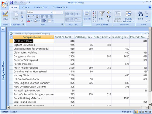
A crosstab query summarizes query results by displaying one field in a table down the left side of the datasheet and additional facts across the top of the datasheet. A crosstab query can, for example, summarize the dollars sold by a salesperson to each company. You can place the name of each company in the query output’s left-most column, and you can display each salesperson across the top. The dollars sold appear in the appropriate cell of the query output (see Figure 12.19).

Figure 12.19. An example of a crosstab query that shows the dollars sold to each company by salesperson.

Crosstab queries are probably one of the most complex and difficult queries to create. For this reason, Microsoft offers a Crosstab Query Wizard. The following sections explain the methods for creating a crosstab query with and without the Crosstab Query Wizard.

Creating a Crosstab Query with the Crosstab Query Wizard

Follow these steps to design a crosstab query with the Crosstab Query Wizard:

1. Select Query Wizard from the Other group on the Create tab.
2. Select Crosstab Query Wizard and click OK.
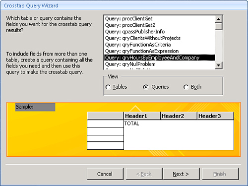
3. Select the table or query that will act as a foundation for the query (see Figure 12-20). If you want to include fields from more than one table in the query, you’ll need to base the crosstab query on another query that has the tables and fields you want. Click Next.

   Figure 12.20. The first step of the wizard asks you to select a table or query on which you want to base the crosstab query.

   

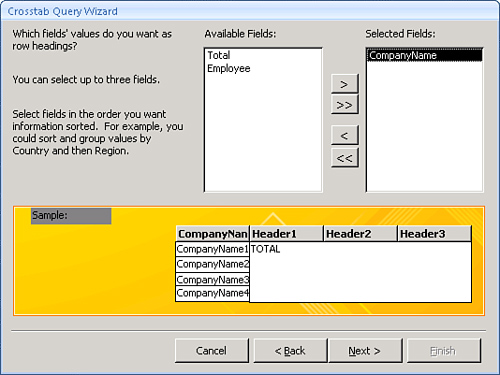
4. Select the fields whose values you want to use as the row headings for the query output. In Figure 12.21, the CompanyName field is selected as the row heading. Click Next.

   Figure 12.21. Specifying the rows of a crosstab query.

   

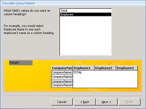
5. Select the field whose values you want to use as the column headings for the query output. In Figure 12.22, the Employee field is selected as the column heading. Click Next.

   Figure 12.22. Specifying the columns of a crosstab query.

   

6. The Crosstab Query Wizard asks you to specify what field stores the number you want to use to calculate the value for each column and row intersection. In Figure 12.23, the Total field is totaled for each company and employee. Click Next.

   Figure 12.23. Specifying the field you want the crosstab query to use for calculating.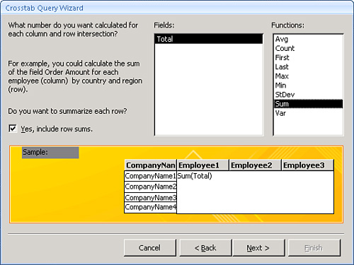

   

7. Specify a name for your query. When you’re done, click Finish.

Figure 12.24 shows a completed crosstab query in Design view; take a look at several important attributes. Notice the Crosstab row of the query grid. The CompanyName field is specified as the row heading and is used as Group By columns for the query. The Employee field is included as a column heading; it is also used as a Group By for the query.

Figure 12.24. A completed crosstab query in Design view.

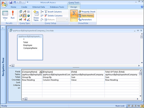
The Total is specified as a value. The Total cell for the column indicates that this field will be summed (as opposed to being counted, averaged, and so on).

Notice the column labeled Total of Total. This column displays the total of all the columns in the query. It’s identical to the column containing the value except for the alias in the field name and the fact that the Crosstab cell is set to Row Heading rather than Value.

Creating a Crosstab Query Without the Crosstab Query Wizard

Although you can create many of your crosstab queries by using the Crosstab Query Wizard, you should know how to build one without the wizard. This knowledge lets you modify existing crosstab queries and gain ultimate control over creating new queries.

To build a crosstab query without using the Crosstab Query Wizard, follow these steps:

1. Click Query Design in the Other group on the Create tab.
2. Select the table or query that will be included in the query grid. Click Add to add the table or query. Click Close.
3. Select Crosstab from the Query Type group on the Design tab.
4. Add to the query grid the fields you want to include in the query output.
5. Click the Crosstab row of each field you want to include as a row heading. Select Row Heading from the drop-down list.
6. Click the Crosstab row of the field you want to include as a column heading. Select Column Heading from the drop-down list.
7. Click the Crosstab row of the field whose values you want to cross-tabulate. Select Value from the Crosstab drop-down list.
8. Select the appropriate aggregate function from the Total drop-down list.
9. Add any date intervals or other expressions you want to include.
10. Specify any criteria for the query.
11. Change the sort order of any of the columns, if you like.
12. Run the query when you’re ready.

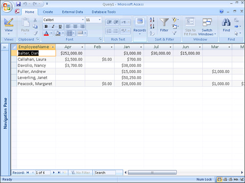
Figure 12.25 shows a query in which the column heading is set to the month of the ProjectBeginDate field; the row heading is set to the EmployeeName field. The sum of the ProjectTotalEstimate field is the value for the query. The ProjectBeginDate is also included in the query grid as a WHERE clause for the query. Figure 12.26 shows the results of running the query.

Figure 12.25. A crosstab query, designed without a wizard, showing the project total estimate by employee and month.

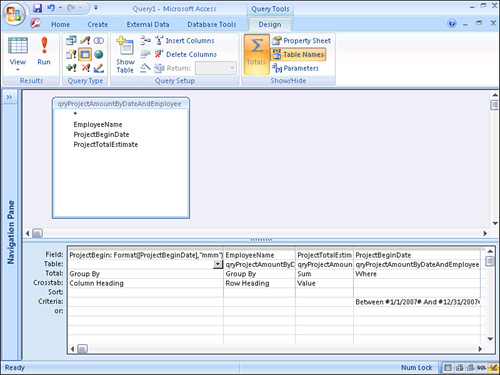
Figure 12.26. The result of running the crosstab query shown in Figure 12.25.

Creating Fixed Column Headings

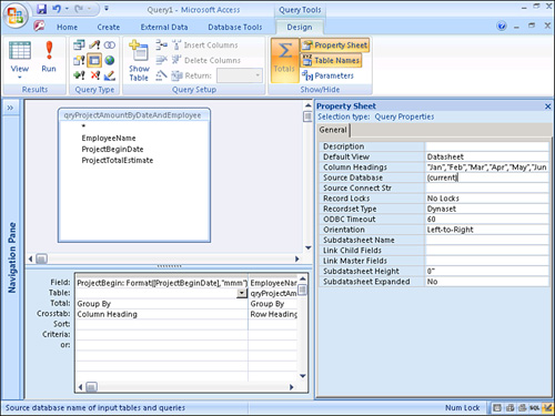
If you don’t use fixed column headings, all the columns are included in the query output in alphabetical order. For example, if you include month names in the query result, they appear as Apr, Aug, Dec, Feb, and so on. By using fixed column headings, you tell Access the order in which each column appears in the query result. You can specify column headings by setting the query’s Column Headings property (see Figure 12.27).

Figure 12.27. A query’s Column Headings property.

Important Notes About Crosstab Queries

Regardless of how crosstab queries are created, you should be aware of some special caveats when working with them:

• You can select only one value and one column heading for a crosstab query, but you can select multiple row headings.
• The results of a crosstab query can’t be updated.
• You can’t define criteria on the Value field. If you do, you get the error message You can't specify criteria on the same field for which you enter a Value in the Crosstab row. If you must specify criteria for the Value field, you must first build another query that includes your selection criteria and base the crosstab query on the first query.
• All parameters used in a crosstab query must be explicitly declared in the Query Parameters dialog box.

Establishing Outer Joins

You use outer joins when you want the records on the one side of a one-to-many relationship to be included in the query result, regardless of whether there are matching records in the table on the many side. With a Customers table and an Orders table, for example, users often want to include only customers with orders in the query output. An inner join (the default join type) does this. In other situations, users want all customers to be included in the query result, whether or not they have orders. This is when an outer join is necessary.

To establish an outer join, you must modify the join between the tables included in the query:

1. Double-click the line joining the tables in the query grid.
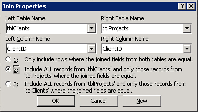
2. The Join Properties window appears (see Figure 12.28). Select the type of join you want to create. To create a left outer join between the tables, select Option 2 (Option 3 if you want to create a right outer join). Notice in Figure 12.28 that the description is Include ALL Records from tblClients and Only Those Records from tblProjects Where the Joined Fields Are Equal.

   Figure 12.28. Establishing a left outer join.

   

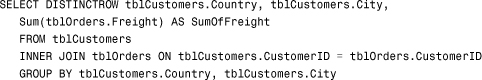
3. Click OK to accept the join. An outer join should be established between the tables. Notice that the line joining the two tables now has an arrow pointing to the many side of the join.

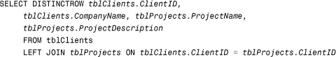
The SQL statement produced when a left outer join is established looks like this:

SELECT DISTINCTROW tblClients.ClientID, tblClients.CompanyName
FROM tblClients
LEFT JOIN tblProjects ON tblClients.ClientID = tblProjects.ClientID;

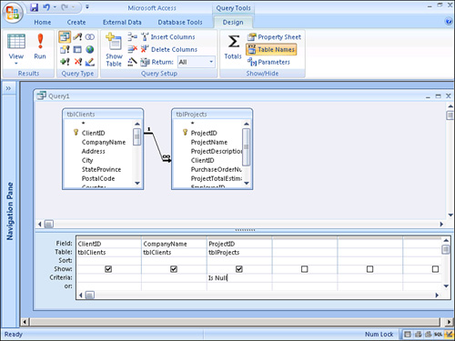
A left outer join can also be used to identify all the records on the “one” side of a join that don’t have corresponding records on the “many” side. To do this, simply enter Is Null as the criterion for any required field on the “many” side of the join. A common solution is to place the criterion on the foreign key field. In the query shown in Figure 12.29, only clients without projects are displayed in the query result.

Figure 12.29. A query showing clients without projects.

Establishing Self-Joins

A self-join enables you to join a table to itself. This is often done so that information in a single table can appear to exist in two separate tables. A classic example is seen with employees and supervisors. Two fields are included in the Employees table: One field includes the EmployeeID of the employee being described in the record, and the other field specifies the EmployeeID of the employee’s supervisor. If you want to see a list of employee names and the names of their supervisors, you’ll need to use a self-join.

To build a self-join query, follow these steps:

1. Click the Query Design button in the Other group on the Create tab.
2. From the Show Tables dialog box, add the table to be used in the self-join to the query grid two times. Click Close. Notice that the second instance of the table appears with an underscore and the number 1.
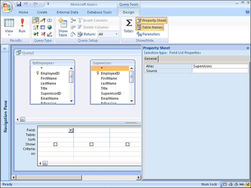
3. To change the alias of the second table, right-click on top of the table in the query grid and select Properties. Change the Alias property as desired. In Figure 12.30, the alias has been changed to Supervisors.

   Figure 12.30. Building a self-join.

   

4. To establish a join between the table and its alias, click and drag from the field in one table that corresponds to the field in the aliased table. In Figure 12.31, the SupervisorID field of the tblEmployees table has been joined with the EmployeeID field from the aliased table.

   Figure 12.31. Establishing a self-join between the table and its alias.

   

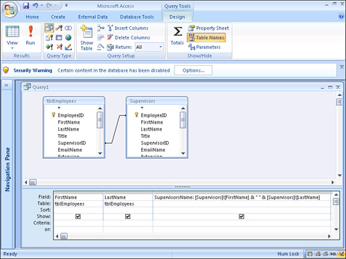
5. Drag the appropriate fields to the query grid. In Figure 12.31, the FirstName and LastName fields are included from the tblEmployees table. The SupervisorName expression (a concatenation of the supervisor’s first and last names) is supplied from the copy of the table with the Supervisors alias.

Understanding SQL

Access SQL is the language that underlies Access queries, so you need to understand a little bit about it, where it came from, and how it works. Access SQL enables you to construct queries without using the Access Query By Example (QBE) grid. This is necessary, for example, if you must build a SQL statement on the fly in response to user interaction with your application. Furthermore, certain operations supported by Access SQL aren’t supported by the graphical QBE grid. You must build these SQL statements in the Query Builder’s SQL view. In addition, many times you will want to build the record source for a form or report on the fly. In those situations, you must have command of the SQL language. Finally, you will want to use SQL statements in your ADO code. For all these reasons, learning SQL is a valuable skill.

What Is SQL, and Where Did It Come From?

SQL is a standard from which many different dialects have emerged. It was developed at an IBM research laboratory in the early 1970s and first formally described in a research paper released in 1974 at an Association for Computing Machinery meeting. Jet 4.0, the version of the Jet Engine provided with Access 2000 and above, has two modes: One supports Access SQL, and the other supports SQL-92. The Access Database Engine, included with Access 2007, also supports the SQL-92 extensions. The SQL-92 extensions are not available from the user interface. They can only be accessed using ADO. They are covered in a later section of this chapter, “Understanding Jet 4.0 ANSI-92 Extensions.”

What Do You Need to Know About SQL?

At the very least, you need to understand SQL’s basic constructs, which enable you to select, update, delete, and append data by using SQL commands and syntax. Access SQL is made up of very few verbs. The sections that follow cover the most commonly used verbs.

SQL Syntax

SQL is easy to learn. When retrieving data, you simply build a SELECT statement. SELECT statements are composed of clauses that determine the specifics of how the data is selected. When they’re executed, SELECT statements select rows of data and return them as a recordset.

The SELECT Statement

The SELECT statement is at the heart of the SQL language. It is used to retrieve data from one or more tables. Its basic syntax is

SELECT column-list FROM table-list WHERE where-clause ORDER BY order-by-clause

The SELECT Clause

The SELECT clause specifies what columns you want to retrieve from the table whose data is being returned to the recordset. The basic syntax for a SELECT clause is

SELECT column-list

The simplest SELECT clause looks like this:

SELECT *

This SELECT clause retrieves all columns from a table. Here’s another example that retrieves only the ClientID and CompanyName columns from a table:

SELECT ClientID, CompanyName

You not only can include columns that exist in your table, but also can include expressions in a SELECT clause. Here’s an example:

SELECT ClientID, City & ", " & State & " " & PostalCode AS Address

This SELECT clause retrieves the ClientID column as well as an alias called Address, which includes an expression that concatenates the City, State, and PostalCode columns.

The FROM Clause

The FROM clause specifies the tables or queries from which the records should be selected. It can include an alias you use to refer to the table. The FROM clause looks like this:

FROM table-list [AS alias]

Here’s an example of a basic FROM clause:

FROM tblClients AS Clients

In this case, the name of the table is tblClients, and the alias is Clients. If you combine the SELECT clause with the FROM clause, the SQL statement looks like this:

SELECT ClientID, CompanyName FROM tblClients

This SELECT statement retrieves the ClientID and CompanyName columns from the tblClients table.

Just as you can alias the fields included in a SELECT clause, you can also alias the tables included in the FROM clause. The alias is used to shorten the name, to simplify a cryptic name, and to perform a variety of other functions. Here’s an example:

SELECT ClientID, CompanyName FROM tblClients AS Customers

This SQL statement selects the ClientID and CompanyName fields from the tblClients table, aliasing the tblClients table as Customers.

The WHERE Clause

The WHERE clause limits the records retrieved by the SELECT statement. You must follow several rules when building a WHERE clause. The text strings that you are searching for must be enclosed in quotation marks. Dates must be surrounded by pound (#) signs. Finally, you must include the keyword LIKE when using wildcard characters. A WHERE clause can include up to 40 columns combined by the keywords AND and OR. The syntax for a WHERE clause looks like this:

WHERE expression1 [{AND|OR} expression2 [...]]

A simple WHERE clause looks like this:

WHERE Country = "USA"

Using an AND to further limit the criteria, the WHERE clause looks like this:

WHERE Country = "USA" AND ContactTitle Like "Sales*"

This WHERE clause limits the records returned to those in which the country is equal to USA and the ContactTitle begins with Sales. Using an OR, the SELECT statement looks like this:

WHERE Country = "USA" OR Country = "Canada"

This WHERE clause returns all records in which the country is equal to either USA or Canada. Compare that with the following example:

WHERE Country = "USA" OR ContactTitle Like "Sales*"

This WHERE clause returns all records in which the Country is equal to USA or the ContactTitle begins with Sales. For example, if the ContactTitle for the salespeople in China begins with Sales, the names of those salespeople will be returned from this WHERE clause. The WHERE clause combined with the SELECT and FROM clauses looks like this:

The ORDER BY Clause

The ORDER BY clause determines the order in which the returned rows are sorted. It’s an optional clause, and it looks like this:

ORDER BY column1 [{ASC|DESC}], column2 [{ASC|DESC}] [,...]]

Here’s an example:

ORDER BY ClientID

The ORDER BY clause can include more than one field:

ORDER BY Country, ClientID

When more than one field is specified, the leftmost field is used as the primary level of sort. Any additional fields are the lower sort levels. Combined with the rest of the SELECT statement, the ORDER BY clause looks like this:

The ORDER BY clause allows you to determine whether the sorted output appears in ascending or descending order. By default, output appears in ascending order. To switch to descending order, use the optional keyword DESC. Here’s an example:

SELECT ClientID, CompanyName FROM tblClients ORDER BY ClientID DESC

This example selects the ClientID and CompanyName fields from the tblClients table, ordering the output in descending order by the ClientID field.

The JOIN Clause

Often you’ll need to build SELECT statements that retrieve data from more than one table. When building a SELECT statement based on more than one table, you must join the tables with a JOIN clause. The JOIN clause differs depending on whether you join the tables with an INNER JOIN, a LEFT OUTER JOIN, or a RIGHT OUTER JOIN.

The SQL-89 and SQL-92 syntax for joins differs. The basic SQL-89 syntax is

SELECT column-list FROM table1, table2 WHERE table1.column1 = table2.column2

The SQL-92 syntax is preferred because it separates the join from the WHERE clause. It is

Note that the keyword OUTER is optional.

Here’s an example of a simple INNER JOIN:

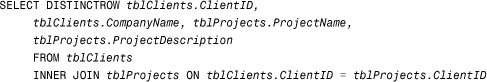
Notice that four columns are returned in the query result. Two columns are from tblClients and two are from tblProjects. The SELECT statement uses an INNER JOIN from tblClients to tblProjects based on the ClientID field. This means that only clients who have projects are displayed in the query result. Compare this with the following SELECT statement:

This SELECT statement joins the two tables using a LEFT JOIN from tblClients to tblProjects based on the ClientID field. All clients are included in the resulting records, whether or not they have projects.

Sometimes you will need to join more than two tables in a SQL statement. When you need to do this, the ANSI-92 syntax is

FROM table1 JOIN table2 ON condition1 JOIN table3 ON condition2

The following example joins the tblClients, tblProjects, and tblPayments tables:

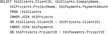
In the example, the order of the joins is unimportant. The exception to this is when inner and outer joins are combined. When combining inner and outer joins, the Access Database Engine applies two specific rules. First, the nonpreserved table in an outer join cannot participate in an inner join. The nonpreserved table is the one whose rows might not appear. In the case of a left outer join from tblClients to tblProjects, the tblProjects table is considered the nonpreserved table. It therefore cannot participate in an inner join with tblPayments. The second rule is that the nonpreserved table in an outer join cannot participate with another nonpreserved table in another outer join.

Self-Joins

Self-joins were covered earlier in this chapter. The SQL syntax required to create them is similar to a standard join and is covered here:

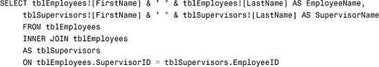
Notice that the tblEmployees table is joined to an alias of the tblEmployees table that is referred to as tblSupervisors. The SupervisorID from the tblEmployees table is joined with the EmployeeID field from the tblSupervisors alias. The fields included in the output are the FirstName and LastName from the tblEmployees table and the FirstName and LastName from the alias of the tblEmployees table.

Non-Equi Joins

So far, all the joins that we have covered involve situations in which the value of a field in one table is equal to the value of the field in the other table. You can create non-equi joins in which the >, >=, <, <=, <>, or Between operator is used to join two tables. Here’s an example:

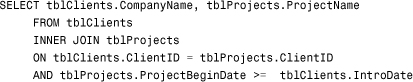
This example returns only the rows from tblProjects where the ProjectBeginDate is on or after the IntroDate stored in the tblClients table.

ALL, DISTINCTROW, and DISTINCT Clauses

The ALL clause of a SELECT statement means that all rows meeting the WHERE clause are included in the query result. When the DISTINCT keyword is used, Access eliminates duplicate rows, based on the fields included in the query result. This is the same as setting the Unique Values property to Yes in the graphical QBE grid. When the DISTINCTROW keyword is used, Access eliminates any duplicate rows based on all columns of all tables included in the query (whether they appear in the query result or not). This is the same as setting the Unique Records property to Yes in the graphical QBE grid. These keywords in the SELECT clause look like this:

SELECT [{ALL|DISTINCT|DISTINCT ROW}] column-list

The TOP Predicate

The Top Values property, available via the user interface, is covered in the “Viewing Special Query Properties” section, earlier in this chapter. The keyword TOP is used to implement this feature in SQL. The syntax looks like this:

SELECT [{ALL|DISTINCT|DISTINCTROW}] [TOP n [PERCENT]] column-list

The example that follows extracts the five clients whose IntroDate field is most recent:

The GROUP BY Clause

The GROUP BY clause is used to calculate summary statistics; it’s created when you build a Totals query by using the graphical QBE grid. The syntax of the GROUP BY clause is

GROUP BY group-by-expression1 [,group-by-expression2 [,...]]

The GROUP BY clause is used to dictate the fields on which the query result is grouped. When multiple fields are included in a GROUP BY clause, they are grouped from left to right. The output is automatically ordered by the fields designated in the GROUP BY clause. In the following example, the SELECT statement returns the country, city, and total freight for each country/city combination. The results are displayed in order by country and city:

The GROUP BY clause indicates that detail for the selected records isn’t displayed. Instead, the fields indicated in the GROUP BY clause are displayed uniquely. One of the fields in the SELECT statement must include an aggregate function. This result of the aggregate function is displayed along with the fields specified in the GROUP BY clause.

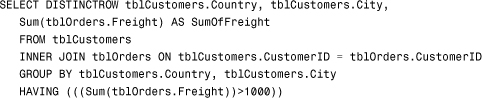
The HAVING Clause

A HAVING clause is similar to a WHERE clause, but it differs in one major respect: It’s applied after the data is summarized rather than before. In other words, the WHERE clause is used to determine which rows are grouped. The HAVING clause determines which groups are included in the output. A HAVING clause looks like this:

HAVING expression1 [{AND|OR} expression2[...]]

In the following example, the criterion > 1000 will be applied after the aggregate function SUM is applied to the grouping:

Applying What You Have Learned

You can practice entering and working with SQL statements in two places:

• In a query’s SQL View window
• In VBA code

In the following sections, you look at both of these techniques.

Using the Graphical QBE Grid as a Two-Way Tool

A great place to practice writing SQL statements is in the SQL View window of a query. It works like this:

1. Start by building a new query.
2. Add a couple of fields and maybe even some criteria.
3. Use the View drop-down list in the Results group of the Design tab to select SQL view.
4. Try changing the SQL statement, using what you have learned in this chapter.
5. Use the View drop-down list in the Results group of the Design tab to select Design view. As long as you haven’t violated any Access SQL syntax rules, you can easily switch to the query’s Design view and see the graphical result of your changes. If you’ve introduced any syntax errors into the SQL statement, an error occurs when you try to return to the query’s Design view.

Including SQL Statements in VBA Code

You can also execute SQL statements directly from VBA code. You can run a SQL statement from VBA code in two ways:

• You can build a temporary query and execute it.
• You can open a recordset with the SQL statement as the foundation for the recordset.

The VBA language enables you to build a query on the fly, execute it, and never store it. The code looks like this:

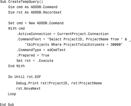
Working with recordsets is covered extensively in Chapter 15. For now, you need to understand that this code creates a temporary query definition using a SQL statement. In this example, the query definition is never added to the database. Instead, the SQL statement is executed but never stored.

A SQL statement can also be provided as part of the recordset’s Open method. The code looks like this:

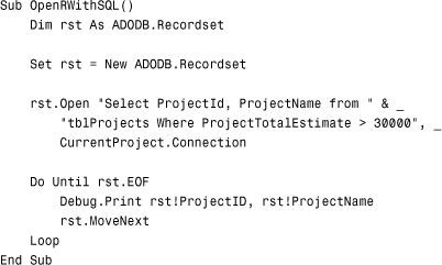
Again, this code is discussed more thoroughly in Chapter 15. Notice that the Open method of the recordset object receives two parameters: The first is a SELECT statement, and the second is the Connection object.

Building Union Queries

A union query enables you to combine data from two tables with similar structures; data from each table is included in the output. For example, suppose you have a tblTimeCards table containing active time cards and a tblTimeCardsArchive table containing archived time cards. The problem occurs when you want to build a report that combines data from both tables. To do this, you must build a union query as the record source for the report. The syntax for a union query is

Here’s an example:

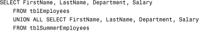
This example combines data from the tblEmployees table with data from the tblSummerEmployees table, preserving duplicate rows, if there are any.

The ALL Keyword

Notice the keyword ALL in the previous SQL statement. By default, Access eliminates all duplicate records from the query result. This means that if an employee is found in both the tblEmployees and tblSummerEmployees tables, he appears only once in the query result. Including the keyword ALL causes any duplicate rows to display.

Sorting the Query Results

When sorting the results of a union query, you must include the ORDER BY clause at the end of the SQL statement. Here’s an example:

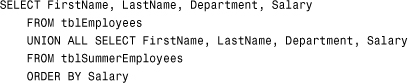
This example combines data from the tblEmployees table with data from the tblSummerEmployees table, preserving duplicate rows, if there are any. It orders the results by the Salary field (combining the data from both tables).

If the column names that you are sorting by differ in the tables included in the union query, you must use the column name from the first table.

Using the Graphical QBE to Create a Union Query

You can use the graphical QBE to create a union query. The process is as follows:

1. Click Query Design in the Other group on the Create tab.
2. Click Close from the Show Tables dialog box without selecting a table.
3. Choose Union Query in the Query Type group on the Design tab. A SQL window appears.
4. Type in the SQL UNION clause. Notice that you can’t switch back to the query’s Design view (see Figure 12.32).

   Figure 12.32. An example of a union query that combines tblTimeCards with tblTimeCardsArchive.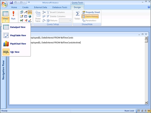

   

5. Click the Run button on the ribbon to execute the query.

Important Notes about Union Queries

It is important to note that the result of a union query is not updateable. Furthermore, the fields in each SELECT statement are matched only by position. This means that you can get strange results by accidentally listing the FirstName field followed by the LastName field in the first SELECT statement, and the LastName field followed by the FirstName field in the second SELECT statement. Each SELECT statement included in a union query must contain the same number of columns. Finally, each column in the first SELECT statement much have the same data type as the corresponding column in the second SELECT statement.

Using Pass-Through Queries

Pass-Through queries enable you to send uninterpreted SQL statements to your back-end database when you’re using something other than the Access Database Engine. These uninterpreted statements are in the SQL that’s specific to your particular back end. Although the Access Database Engine sees these SQL statements, it makes no attempt to parse or modify them. Pass-Through queries are used in several situations:

• The action you want to take is supported by your back-end database server but not by Access SQL or ODBC SQL.
• Access or the ODBC driver is doing a poor job parsing the SQL statement and sending it in an optimized form to the back-end database.
• You want to execute a stored procedure on the back-end database server.
• You want to make sure the SQL statement is executed on the server.
• You want to join data from more than one table residing on the database server. If you execute the join without a Pass-Through query, the join is done in the memory of the user’s PC after all the required data has been sent over the network.

Although Pass-Through queries offer many advantages, they aren’t a panacea. They do have a few disadvantages:

• Because you’re sending SQL statements specific to your particular database server, you must write the statement in the “dialect” of SQL used by the database server. For example, in writing a Pass-Through query to access SQL Server data, you must write the SQL statement in T-SQL. When writing a Pass-Through query to access Oracle data, you must write the SQL statement in PL-SQL. This means that you’ll need to rewrite all the SQL statements if you switch to another back end.
• The results returned from a Pass-Through query can’t be updated.
• The Access Database Engine does no syntax checking of the query before passing it on to the back end.

Now that you know all the advantages and disadvantages of Pass-Through queries, you can learn how to build one:

1. Click Query Design in the Other group on the Create tab.
2. Click Close from the Show Tables dialog box without selecting a table.
3. Choose Pass-Through Query in the Query Type group on the Design tab to open the SQL Design window.
4. Type in the SQL statement in the dialect of your back-end database server.
5. View the Query Properties window and enter an ODBC connect string (see Figure 12.33).

   Figure 12.33. A SQL Pass-Through query that selects specific fields from the Sales table, which resides in the PublisherInfo data source.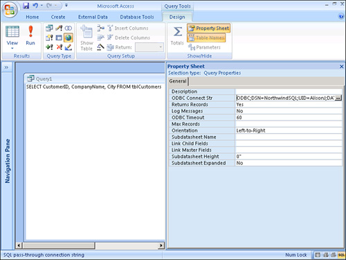

   

6. Click the Run button on the ribbon to run the query.

Examining the Propagation of Nulls and Query Results

Null values can wreak havoc with your query results because they propagate. Look at the query in Figure 12.34. Notice that when parts and labor are added, and either the Parts field or the Labor field contains a Null, the result of adding the two fields is Null. In Figure 12.35, the problem is rectified. Figure 12.36 shows the design of the query that eliminates the propagation of the Nulls. Notice the expression that adds the two values:

TotalPrice: Nz([Parts]) + Nz([Labor])

Figure 12.34. An example that shows the propagation of Nulls in a query result.

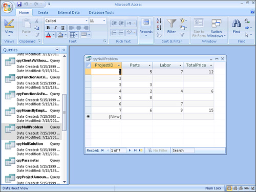
Figure 12.35. An example that shows Nulls eliminated from the query result.

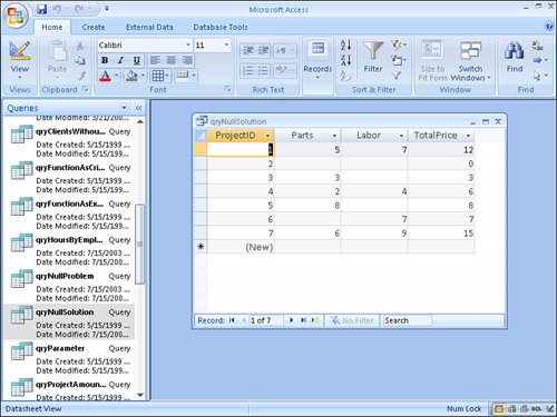
Figure 12.36. A solution to eliminate propagation of Nulls.

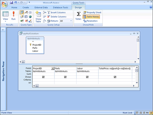
This expression uses the Nz function to convert the Null values to 0 before the two field values are added together.

Running Subqueries

Subqueries allow you to embed one SELECT statement within another. By placing a subquery in a query’s criteria, you can base one query on the result of another. Figure 12.37 shows an example. The query pictured finds all the clients without projects.

Figure 12.37. A query containing a subquery.

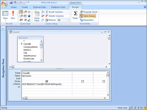
The SQL statement looks like this:

This query first runs the SELECT statement SELECT ClientID from tblProjects. It uses the result as criteria for the first query.

Using SQL to Update Data

SQL can be used not only to retrieve data, but to update it as well. This concept was introduced in the section “Using Action Queries,” which focused on the SQL statements behind the action queries.

The UPDATE Statement

The UPDATE statement is used to modify the data in one or more columns of a table. The syntax for the UPDATE statement is

The WHERE clause in the UPDATE statement is used to limit the rows that are updated. The following is an example of an UPDATE statement:

This statement updates the DefaultRate column of the tblClients table, increasing it by 10% for any clients that have a default rate less than or equal to 125.

The DELETE Statement

Whereas the UPDATE statement is used to update all rows that meet specific criteria, the DELETE statement deletes all rows that meet the specified criteria. The syntax for the DELETE statement is

DELETE FROM table [WHERE criteria]

As with the UPDATE statement, the WHERE clause is used to limit the rows that are deleted. The following is an example of the use of a DELETE statement:

This statement deletes all clients from the tblClients table whose DefaultRate field is less than or equal to 125.

The INSERT INTO Statement

The INSERT INTO statement is used to copy rows from one table to another. The syntax for the INSERT INTO statement is

INSERT INTO target-table select-statement [WHERE criteria]

Once again, the optional WHERE clause is used to limit the rows that are copied. Here’s an example:

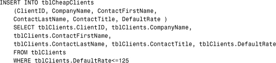
This statement inserts the ClientID, CompanyName, ContactFirstName, ContactLastName, ContactTitle, and DefaultRate fields into the corresponding fields in the tblCheapClients table for any clients whose DefaultRate field is less than or equal to 125.

The SELECT INTO Statement

Whereas the INSERT INTO statement inserts data into an existing table, the SELECT INTO statement inserts data into a new table. The syntax looks like this:

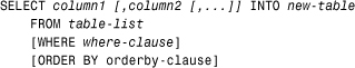
The WHERE clause is used to determine which rows in the source table are inserted into the destination table. The ORDER BY clause is used to designate the order of the rows in the destination table. Here’s an example:

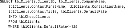
This statement inserts data from the selected fields in the tblClients table into a new table called tblCheapClients. Only the clients whose DefaultRate field is less than or equal to 125 are inserted.

Using SQL for Data Definition

Access 2007 offers two methods of programmatically defining and modifying objects. You can use either ActiveX Data Object Extensions for DDL and Security (ADOX) or Data Definition Language (DDL). DDL is covered in this chapter. ADOX is introduced in Chapter 15.

The CREATE TABLE Statement

As its name implies, the CREATE TABLE statement is used to create a new table. The syntax is

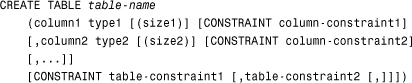
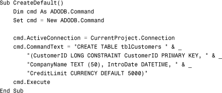
You must designate the type of data for each column included in the table. When defining a text field, you can also specify the size parameter. Notice that constraints are available at the table level and at the field level. Here’s an example of a CREATE TABLE statement:

This example creates a table named tblCustomers. The table will contain three fields: CustomerID (Long), CompanyName (Text), and IntroDate (DateTime).

The CONSTRAINT clause allows you to create primary and foreign keys. It looks like this:

CONSTRAINT name {PRIMARY KEY|UNIQUE|REFERENCES foreign-table [foreign-column]}

Here’s an example:

The example creates a primary key index based on the CustomerID field.

The CREATE INDEX Statement

The CREATE INDEX statement is used to add an index to an existing table. It is supported in Access but is not part of the ANSI standard. It looks like this:

Here’s an example:

The example creates an index called CompanyName, based on the CompanyName field.

The ALTER TABLE Statement

The ALTER TABLE statement is used to modify the structure of an existing table. The syntax has four forms. The first form looks like this:

ALTER TABLE table-name ADD [COLUMN] column-name datatype [(size)]
[CONSTRAINT column-constraint]

This form of the ALTER TABLE statement adds a column to an existing table. Here’s an example:

ALTER TABLE tblCustomers ADD ContactName Text 50

The second form uses the following syntax to delete a column from an existing table:

ALTER TABLE table-name DROP [COLUMN] column-name

Here’s an example:

ALTER TABLE tblCustomers DROP COLUMN ContactName

The third form uses the ALTER TABLE statement to add a constraint to an existing column. The syntax is

ALTER TABLE table-name ADD CONSTRAINT constraint

Here’s an example:

ALTER TABLE tblCustomers ADD CONSTRAINT CompanyName UNIQUE (CompanyName)

Finally, the fourth form drops a constraint from an existing column:

ALTER TABLE table-name DROP CONSTRAINT index

Here’s an example:

ALTER TABLE tblCustomers DROP CONSTRAINT CompanyName

The DROP INDEX Statement

The DROP INDEX statement is used to remove an index from a table. The syntax is as follows:

DROP INDEX index ON table-name

Here’s an example:

DROP INDEX CompanyName ON tblCustomers

The DROP TABLE Statement

The DROP TABLE statement is used to remove a table from the database. The syntax is

DROP TABLE table-name

Here’s an example:

DROP TABLE tblCustomers

Using the Result of a Function as the Criteria for a Query

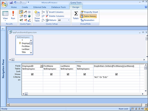
Many people are unaware that the result of a function can serve as an expression in a query or as a parameter to a query. The query shown in Figure 12.38 evaluates the result of a function called Initials. The return value from the function is evaluated with criteria to determine whether the employee is included in the query result. The Initials function shown here (it’s also in the basUtils module of CHAP12EX.ACCDB, found on the sample code website) receives two strings and returns the first character of each string followed by a period:

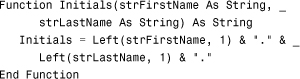
Figure 12.38. A query that uses the result of a function as an expression.

The return value from a function can also be used as the criteria for a query (see Figure 12.39). The query in the figure uses a function called HighlyPaid to determine which records appear in the query result. Here’s what the HighlyPaid function looks like. (It’s also in the basUtils module of CHAP12EX.ACCDB, found on the sample code website.)

Figure 12.39. A query that uses the result of a function as criteria.

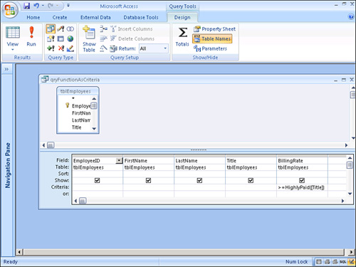
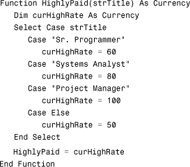
The function receives the employee’s title as a parameter. It then evaluates the title and returns a threshold value to the query that’s used as the criterion for the query’s Billing Rate column.

Passing Parameter Query Values from a Form

The biggest frustration with Parameter queries occurs when multiple parameters are required to run a query. The user is confronted with multiple dialog boxes, one for each parameter in the query. The following steps explain how to build a Parameter query that receives its parameter values from a form:

1. Create a new unbound form.
2. Add text boxes or other controls to accept the criteria for each parameter added to your query.
3. Name each control so that you can readily identify the data it contains.
4. Add a command button to the form and instruct it to call the Parameter query (see Figure 12.40).

   Figure 12.40. The Click event code of the command button that calls the Parameter query.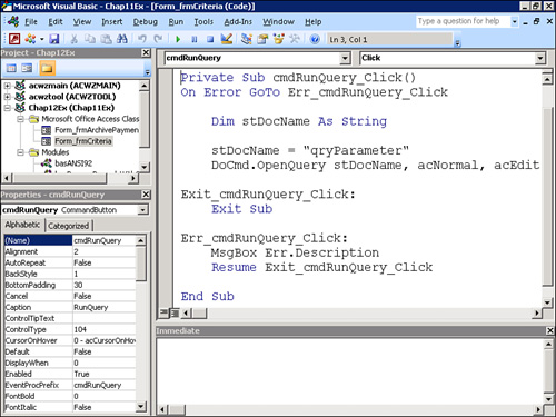

   

5. Save the form.
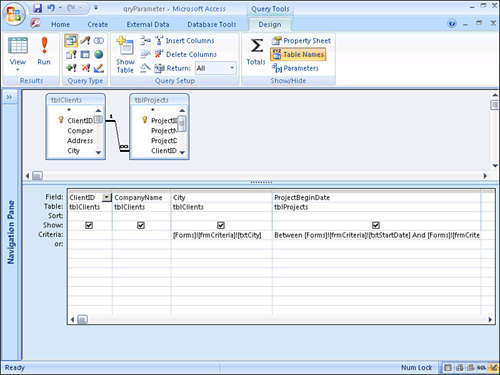
6. Create the query and add the parameters to it. Each parameter should refer to a control on the form (see Figure 12.41).

   Figure 12.41. Parameters that refer to controls on a form.

   

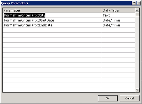
7. Right-click the top half of the Query Design grid and select Parameters. Define a data type for each parameter in the Query Parameters dialog box (see Figure 12.42).

   Figure 12.42. The Query Parameters dialog box lets you select the data type for each parameter in the query.

   

8. Save and close the query.
9. Fill in the values on the criteria form and click the command button to execute the query. It should execute successfully.

Understanding Jet 4.0 ANSI-92 Extensions

Jet 4.0, the version of Jet that ships with Access 2000 and later, includes expanded support for the ANSI-92 standard. The Access Database Engine, included with Access 2007, supports these same features. Although these extensions are not available via the Access user interface, you can tap into them using ADO code. The following sections cover the extensions and the functionality they afford you. Because I have not yet covered ADO, you might want to refer to Chapter 15 to better understand the examples. For now, you need to understand that the code examples in the following sections use the ADO Command object to execute SQL statements that create and manipulate database objects.

Table Extensions

Six table extensions are included with the Access Database Engine. These extensions enable you to

• Create defaults
• Create check constraints
• Set up cascading referential integrity
• Control fast foreign keys
• Implement Unicode string compression
• Better control autonumber fields

Creating Defaults

The DEFAULT keyword can be used with the CREATE TABLE statement. The syntax is

DEFAULT (value)

Here’s an example:

Notice first that ADO is used to execute the SQL statement. The reason is that the DEFAULT keyword is not accessible via the use interface. The CreditLimit field includes a DEFAULT clause that sets the default value of the field to 5000.

Creating Check Constraints

The CHECK keyword can be used with the CREATE TABLE statement. It allows you to add business rules for a table. Unlike field- and table-level validation rules that are available via the user interface, check constraints can span tables. The syntax for a check constraint is

[CONSTRAINT [name]] CHECK (search_condition)

Here’s an example:

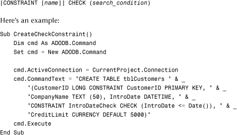
This example creates a check constraint on the IntroDate field that limits the value entered in the field to a date on or before today’s date.

Implementing Cascading Referential Integrity

The ANSI-92 extensions can also be used to establish cascading referential integrity. The syntax is

CONSTRAINT name FOREIGN KEY (column1 [,column2 [,...]])
REFERENCES foreign-table [(foreign-column1 [, foreign-column2 [,...]])]
[ON UPDATE {NO ACTION|CASCADE}]
[ON DELETE {NO ACTION|CASCADE}]

Without the CASCADE options, the primary key field cannot be updated if the row has child records, and the row on the “one” side of the one-to-many relationship cannot be deleted if it has children.

Controlling Fast Foreign Keys

Whenever you join two tables in a one-to-many relationship, Access automatically creates an index on the foreign key field (the “many” side of the relationship). This is generally a good thing. It is bad only if the foreign key contains a lot of Nulls. In that case, the index serves only to degrade performance rather than improve it. Fortunately, using the Jet 4.0 or the Access Database Engine ANSI-92 extensions and the NO INDEX keywords, you can create the foreign key without the index. Here’s the syntax:

CONSTRAINT name FOREIGN KEY NO INDEX (column1 [,column2 [,...]])
REFERENCES foreign-table [(foreign-column1 [, foreign-column2 [,...]])]
[ON UPDATE {NO ACTION|CASCADE}]
[ON DELETE {NO ACTION|CASCADE}]

Implementing Unicode String Compression

Just as you can implement Unicode string compression using the user interface, you can also implement it in code. The syntax is

Column string-data-type [(length)] WITH COMPRESSION

Controlling Autonumber Fields

Using the Jet 4.0 or the Microsoft Access Database ANSI-92 extensions, you can change both the autonumber seed and increment. The syntax is

Column AUTOINCREMENT (seed, increment)

Here’s an example:

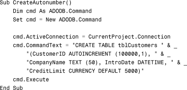
The code creates an auto-increment field called CustomerID. The starting value is 100000. The field increments by 1. In addition to the added support for seed value and increment value, the Jet 4.0 or Access Database Engine ANSI-92 extensions allow you to retrieve the last-assigned autonumber value. Here’s how it works:

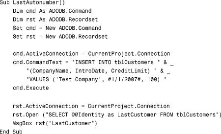
The code first inserts a row into the tblCustomers table. It then opens a recordset and retrieves the @@Identity value. As with SQL Server, this @@Identity variable contains the value of the last assigned autonumber.

View and Stored Procedures Extensions

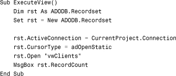
The Jet 4.0 or Access Database Engine ANSI-92 extensions allow you to create views and stored procedures similar to those found in SQL Server. Essentially, these views and stored procedures are Access queries that are repackaged to behave like their SQL Server counterparts. Although stored as queries, the views and stored procedures that you create are not visible via the user interface. You can execute them just like saved queries. The syntax to create a view looks like this:

CREATE VIEW view-name [(field1 [(,field2 [,...]])] AS select-statement

Here’s an example:

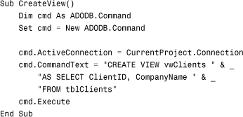
As covered in Chapter 15, use the following code to execute the view:

The syntax to create a stored procedure is

CREATE PROC[EDURE] procedure [(param1 datatype1 [,param2 datatype2 [,...]])]_
AS sql-statement

Here’s an example:

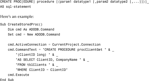
Use the EXECUTE statement, as shown in the following code, to execute the stored procedure:

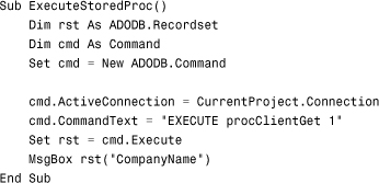
Transaction Extensions

Using Jet 4.0 or Access Database Engine ANSI-92 security extensions, you can create transactions that span an ADO connection. These extensions are intended to augment, rather than replace, ADO transactions. You use BEGIN TRANSACTION to start a transaction, COMMIT TRANSACTION to commit a transaction, and ROLLBACK [TRANSACTION] to cancel a transaction. Transactions are covered in detail in Alison Balter’s Mastering Access 2002 Enterprise Development.

Practical Examples: Applying These Techniques in Your Application

The following sections provide several practical applications of the advanced techniques learned in this chapter.

Archiving Payments

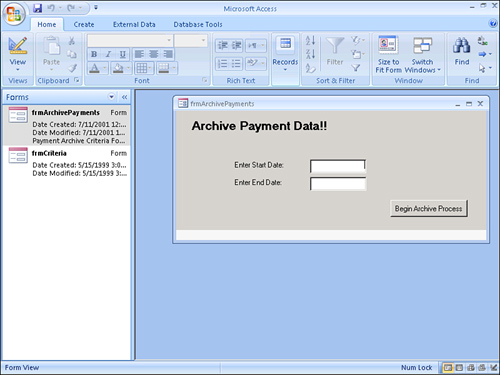
After a while, you might need to archive some of the data in the tblPayment table. Two queries archive the payment data. The first, called qappAppendToPaymentArchive, is an append query that sends all data in a specified date range to an archive table called tblPaymentsArchive (see Figure 12.43). The second query, called qdelRemoveFromPayments, is a delete query that deletes all the data archived from the tblPayments table (see Figure 12.44). The archiving is run from a form called frmArchivePayments, where the date range can be specified by the user at runtime (see Figure 12.45).

Figure 12.43. The append query qappAppendToPaymentArchive.

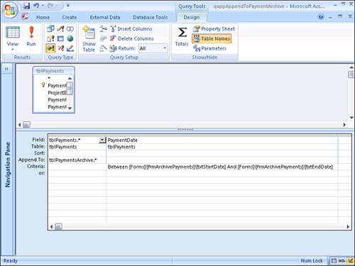
Figure 12.44. The delete query qdelRemoveFromPayments.

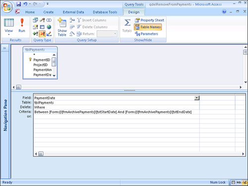
Figure 12.45. The form that supplies criteria for the archive process.

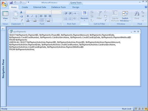
Showing All Payments

At times, you might want to combine data from both tables. To do this, you’ll need to create a union query that joins tblPayments to tblPaymentsArchive. The query’s design is shown in Figure 12.46.

Figure 12.46. Using a union query to join tblPayments to tblPaymentsArchive.

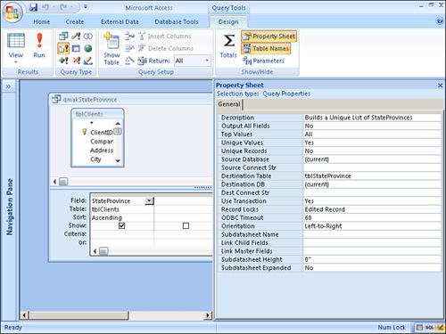
Creating a State Table

Because you’ll regularly be looking up the states and provinces, you need to build a unique list of all the states and provinces in which your clients are currently located. The query needed to do this is shown in Figure 12.47. The query uses the tblClients table to come up with all the unique values for the StateProvince field. Here, you use a make table query that takes the unique list of values and outputs it to a tblStateProvince table.

Figure 12.47. A make table query that creates a tblStateProvince table.

Summary

As you can see, Microsoft gives you a sophisticated query builder for constructing complex and powerful queries. Action queries let you modify table data without writing code; you can use these queries to add, edit, or delete table data. The Unique Values and Top Values properties of a query offer you flexibility in determining exactly what data is returned in your query result.

You can do many things to improve your queries’ efficiency. A little attention to the details covered in this chapter can give you dramatic improvements in your application’s performance.

Other special types of queries covered in this chapter include crosstab queries, outer joins, and self-joins. Whatever you can’t do by using the graphical QBE grid, you can accomplish by typing the required SQL statement directly into the SQL View window. In this window, you can type Access SQL statements or use SQL Pass-Through to type SQL statements in the SQL dialect that’s specific to your back-end database. After you harness the power of the SQL language, you can perform powerful tasks such as modifying the record source of a form or report at runtime.