

1.1 The Nature of NEC-2
It is important to recognize that the Numerical Electromagnetics Code (NEC) is no magic tool—it does some things very well but it cannot do other things. In spite of this, it is a valuable tool that makes a significant contribution to easing the design and adjustment of medium-frequency (MF) broadcast directional antennas.
The user of NEC-2 should have realistic expectations, and recognize from the outset, that the results of a NEC-2 analysis are, at best, an approximation, and they are not necessarily exact answers. Fortunately, however, the results of a NEC-2 analysis need not be precise to be beneficial.
1.2 The Directional Antenna Adjusting Process
The process of physically adjusting the network components of an array to achieve a desired pattern is very similar to that of mathematically synthesizing a radiation pattern using computerized optimizing methods. Both processes start with a given pattern, compare it to a target, determine an error, and then make parameter adjustments in an attempt to reduce the error. In the physical adjustment process, the pattern error is a matter of human opinion; in the case of computerized pattern synthesis, the error is defined mathematically.
The mathematical synthesis process and the physical adjustment process possess the same significant limitation in that neither can know when the minimum error has actually been reached. Therefore, in both cases the usual practice is to test a potential error minimum by changing a parameter value and noting the effect on the error. If the error increases, then the parameter is returned to its original value and another parameter value is changed. If all the parameter values are changed in turn and none reduces the error, then it is often assumed that the error is at a minimum.
The task does not end there, however. The error may indeed be at a minimum, but it may not be at the absolute minimum. There may be another set of parameters that will create an even smaller error. That concept can be better understood by considering the following analogy.
1.3 Local and Global Minima
The pattern error can be envisioned as an N + 1 dimension surface where N is the number of variables.
Figure 1-1 shows a three-dimensional error surface of two variables, arbitrarily called Field Ratio and Phase for example purposes. Point S in Figure 1-1 is taken as an arbitrary starting point from which we
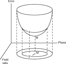
FIGURE 1-1![]()
Error surface of two variables.
will make a search in an effort to find point M, which is the point on the surface representing the values of Field Ratio and Phase where the error is least.
The object is to change the values of Field Ratio and Phase so as to move from point S to point M. That is not necessarily a simple task, especially if there are more than two variables. One must know not only which variable to change, but also the direction of the change and how much change is required. Ultimately, however, after a number of changes, a point will be reached where an additional change of either variable will cause the error to increase. It might then be concluded that point M has been reached.
Only the simplest arrays have smooth error surfaces, as shown in Figure 1-1. The more complex arrays are pock-marked with variations that may be viewed as downward-pointing dimples in the surface. These dimples press the surface down for a range then allow it to rise again. Figure 1-2 shows such a dimple but, for the sake of simplicity, only a one-variable error curve is shown.
Again point S is the starting point in the search for the minimum at point M. Notice, however, that to follow the curve from point S to point M, one must go through point D. While point D suggests that it is the minimum (i.e., at point D the error increases if the variable is varied in either direction), the reduced error at point D is larger than the error at point M. Point M is unique; that is, there can be only one point of least error, so point M is called the global minimum. Point D, on the other hand, is not unique because there can be several points of this type. Therefore, points such as D are called local minima. When adjusting a
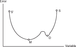
FIGURE 1-2![]()
Single-variable error curve containing a local minimum.
directional array to a target pattern, then in essence, one must journey along the error surface attempting to reach the global minimum. If the error surface does not continuously increase or decrease but instead has a number of dimples, then one may well fall into a dimple and be in a local minimum. Unfortunately, it is not possible to know that it is a local minimum, nor is there a way to determine that it is a local minimum.
Usually, if the error in a minimum is tolerable, then the adjustment process will be stopped, notwithstanding whether the minimum is local or global. This happens more often than not when physically adjusting a complex array.
If the error in the local minimum is intolerable, however, then a new starting point must be chosen and a new adjustment process started from there, hoping to bypass any local minima. For example, if the starting point in Figure 1-2 is changed from point S to point S', it is obvious that the journey along the curve to point M will occur without complications.
1.4 The Role of NEC-2
The idea to convey here is that if the array is simple, then the error surface is likely to be smooth and the probability of reaching the global minimum is high. If the array is complex, however, then the error surface may contain several local minima and the probability of reaching the target without falling into a local minimum is practically zero; so the search process must be repeated over and over … unless the starting point is initially chosen to be very near the global minimum. This is where NEC-2 makes its contribution.
In most cases, a NEC-2 analysis will define a set of starting parameter values that, although they may not necessarily be exact, they are sufficiently accurate to be near enough to the global minimum to avoid most local minima. Therefore, the engineer can initially set the array component values to those determined by a NEC-2 calculation then manually adjust the array to the global minimum without being trapped by a local minimum. This benefit of knowing where to set the parameters in preparation for an initial start-up of a new array can save thousands of dollars in fieldwork. The case histories in later chapters of this book give vivid demonstrations of this benefit.
1.5 Analysis Overview
Unless the reader has previous knowledge of the use of NEC-2, it is not likely that the following steps for NEC-2 analysis will be self-explanatory. Nevertheless, the procedure is presented here as an overview to let the reader know what to expect and what the explanations that follow are seeking to accomplish. So if questions remain after finishing this section, be patient; more detail will be revealed in later chapters.
When using the public domain software furnished on the CD included with this book, it is necessary to make three separate NEC-2 runs to arrive at the NEC-2 output file that yields the final analysis. Fortunately, this is not difficult; nor is it excessively time consuming and the results are just as valuable as those obtained with any commercial software that might have a more user-friendly interface. The NEC-2 computations are made using a slightly modified version of the public domain NEC-2 program called bnec.exe (included on the CD with this book).
The sequence leading to a NEC-2 analysis proceeds according to the following steps.
- Create a NEC-2 unity drive input file that excites each tower individually with 1.0 + j0 volts while the companion towers are grounded. Using that unity drive file as the input file, run bnec.exe.
- Using the NEC-2 output file created by step 1, run the NecDrv.exe computer program included on the associated disk to determine the normalized base drive voltages corresponding to the target field ratios.
- Create a NEC-2 normalized drive input file that excites the towers simultaneously with the normalized base drive voltages determined in step 2. Run bnec.exe with that normalized drive file as the input file.
- Using the NEC-2 output file created by step 3, run the NecMom.exe program included on the associated disk to confirm that the normalized base drive voltages do, in fact, create the target field ratios.
- Scale the normalized base drive voltages determined in step 2 to the full power level (described in Chapter 6 of this book) to generate the desired power output.
- Create a NEC-2 full-power drive input file that excites the towers simultaneously with the full-power base drive voltages determined in step 5. Using that full-power drive file as the input file, run bnec.exe.
- The NEC-2 output file created by step 6 contains the final data for analysis.
Later chapters in this book will show how to interpret the output file to learn the peak values of voltages and current at significant points in the system plus how to read the operating drive point impedance of each tower. Armed with this information, the engineer may calculate the antenna-matching networks and set the individual network component values to a reasonable starting value in preparation for the initial turn-on of the array.
Perhaps the most beneficial result of a NEC-2 analysis is the current distribution listing for each tower of the array. From these current distribution listings, the designer can determine at what height to position the antenna monitor sampling loops such that the antenna monitor will give indications that closely correspond to the associated far-field ratios. He can also determine the base voltage ratios corresponding to the target field ratios if his antenna monitor samples those voltages.
If the sample loops are not positioned at the optimum height, or if current transformers are used to sample the tower current, then the NEC-2 current distribution listing can be used to determine the monitor reading that corresponds to the desired far-field ratio.
Thus, with some indication of the radiated far-field ratios at hand during the initial adjustment process, the array networks can be adjusted to very near their final values without the benefit of distant-field strength measurements and without being plagued by falling into a local minimum.
1.6 Additional NEC-2 Benefits
In addition to defining a suitable set of starting parameters, later chapters will show that the NEC-2 analysis serves several other useful purposes. First, a NEC-2 analysis allows the engineer to explore physical arrangements that are not practical using hardware—the effects of different tower heights, for example. In addition, the engineer is able to examine the impact of unused towers and other structures in the vicinity of the array. He or she is able to study the effects of top loading and tower skirts, as well as shunting reactance at the tower insulator. NEC-2 also gives good indications of power budget, currents, impedances, and so on. In summary, the results obtained from the NEC-2 analysis may not be exact, but they still provide the engineer with an insight into array performance that minimizes the “cut-and-try” effort so common to array adjustment.
1.7 Software Requirements
Antenna analysis software sells for as much as $2000 or more and many of the commercial computer programs being sold for that purpose use the basic NEC-2 or NEC-4 engine. They differ, for the most part, only in the way they present a convenient or novel user interface.
Therefore, in the interest of economy, this book uses the NEC-2 public domain software that can be downloaded from the Internet free of charge. The human interface with the public domain software may not be as elegant as some of the purchased products, and the public domain software may not be as user-friendly, but the results are just as useful and just as rewarding, and the time spent in learning to use it is indeed invested wisely.
If, however, the reader already possesses commercial software, then in most cases the commercial software can be used in lieu of the public domain software. The concepts presented in this book are valid independently of the software used. And while the postprocessing programs furnished on the associated disk may not be compatible with the output format of the commercial software, sufficient information is furnished in the book to allow one to write simple postprocessing programs that are compatible with the output files at hand.