
5.1 Modeling Impedance Loads
Modeling lumped R-L-C impedance loads on one or more segments of a wire is accomplished using the LD command. Series and parallel circuits can be generated in addition to a finite wire conductivity. To review the syntax of the LD command, see the description in Appendix A.
Here is a typical broadcast application:
More often than not, the LD command is used by setting I1 = 0 to add a series impedance to a wire such as might be found in the inductance of a lead or the loss resistance of a wire. It is also commonly used to create an open circuit that is shunted by a capacitor such as might exist at the base insulator of the tower. The finite Q of an inductance can be represented by the LD command with I1 = 0 by showing both R and L in series.
The setting I1 = 1 places a parallel R-L-C circuit in series with a wire. This might be used to represent the shunting effect of the lighting choke in parallel with the base insulator capacity or perhaps a parallel resonant L-C trap in a wire.
Setting I1 equal to other values is less common in broadcast applications, although it is conceivable that one might want to represent tower loss by modeling the tower appropriately and setting I1 = 5 to specify the conductivity of the tower steel. See Appendix A for full details on using the LD command.
The setting I2 identifies the tag number of the wire containing the load. Settings I3 and I4 indicate the segments of that tag receiving the load. If I4 is equal to I3, then the load is placed only in the segment identified by I3. I4 can be greater (but not less) than I3, in which case the LD command will place the specified load in every segment between I3 and I4 inclusive. This feature can be used to model guy wires in which the break-up insulators are represented by a small capacitor that is placed in segments of the guy wire that are of a length equal to the insulator spacing.
The floating-point numbers in the LD command define the value of the R-L-C components in that order. A zero in any R-L-C field indicates that no component is present as opposed to a zero value for that component. For example, in a series R-L-C circuit (LD 0 …), a zero value is the same as a short circuit; in a parallel R-L-C circuit (LD 1 …), a zero value is the same as an open circuit. If a zero value for the component is desired, then a very small number must be entered, such as 1.0E-10.
When an inductance or capacity is entered on an LD command, the resulting reactance is automatically scaled as frequency changes. When reactance is entered on the LD command (I1 =4), the reactance is not automatically scaled with frequency.
Load commands are normally input in groups to achieve a desired structure loading. If a segment is loaded more than once by a group of loading commands, the loads are assumed to be in series.
When a load is placed in a segment that also carries a voltage source, the load appears on the segment in series with the voltage source. If it is desired to have the load appear on the segment in parallel with the voltage source, as might be the case when applying the voltage across the capacity of a base insulator, then the LD command cannot be used. In that case, the NT network command is used.
5.2 Modeling Nonradiating Networks
The NT command generates a two-port nonradiating network connected between specified segments of the structure. Since the network is nonradiating, the physical location of the segments to which the network connects is irrelevant in terms of how the network operates.
The network can be made up of R-L-C components with the network characteristics being specified by its short-circuit admittance matrix parameters. Typical network uses include impedance matching and phasing networks, but more useful applications in a NEC-2 analysis include special kinds of shunt impedance loads and methods for generating tower feeds. The reader is encouraged to review the syntax of the NT card in Appendix A.
Here is a typical broadcast application:
The entries I1 and I2 identify the wire tag and segment number to which port 1 of the network is connected. Entries I3 and I4 identify the wire tag and segment number to which port 2 of the network is connected. The network is described in terms of its complex short-circuit admittance parameters, Y11, Y12, and Y22. The entries Y11R and Y11I in the NT command are the real and imaginary parts of Y11. Y12R and Y12I are the real and imaginary parts of Y12. And Y22R and Y22I are the real and imaginary parts of Y22.
Figure 5-1 shows a two-port network. The Y-parameters are calculated in the usual way.
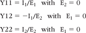
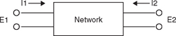
FIGURE 5-1![]()
General two-port network.
It is important to recognize that the Y-parameters do not scale with frequency, and they must be recalculated and repeated for each frequency.
5.2.1 Typical Networks
Figure 5-2 shows the network configuration of some networks commonly used in broadcasting. The following are Y-parameters for the networks in Figure 5-2:
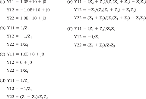
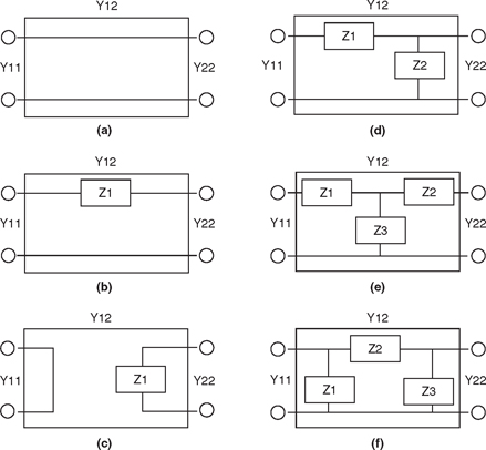
FIGURE 5-2![]()
Common network configurations.
5.2.2 Typical Network Applications
The networks shown in Figure 5-2 are often used as follows:
Network (a) is a pass-through network generally for combining or for use during an analytical in/out comparison of another network.
Network (b) is useful to place an impedance in series with the drive signal, such as to simulate the effect of the small resistance of the spring clips or to include the inductance of the tower lead-in.
Network (c) is used to place an impedance in parallel with a source voltage. Recall that when the LD command is used to place a load in a segment that also carries a voltage source, that load appears on the segment in series with the voltage source. However, when a NT command is used to place a network in a segment that also carries a voltage source, that network appears on the segment in parallel with the voltage source.
For this application, a dummy segment may be defined to accept port 1 of the network. Port 2 will connect to the segment that carries the voltage source. The dummy segment is made to be nonradiating by making it very small and placing it in a far-off location.
An input file that places a drive voltage across a base insulator having 100 pf shunt capacity would contain all the normal commands plus the following:
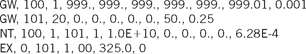
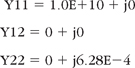
The first GW command creates the dummy segment as segment 1 of the wire having tag 100. The wire is located far away (999.,999.,999); it is vertical and very small (0.01 meter high with 0.001 meter radius). The second GW command creates the driven tower radiator having the wire tag 101 and 20 segments. The NT command connects the network between wire tag 100, segment 1 and wire tag 101, segment 1. The Y-parameters of the network are:
The EX command places the drive voltage in parallel with the network on wire tag 100, segment 1.
Network (d) is used to include both a series impedance and a shunt impedance in the drive path. This might represent the series inductance of a tower feed and the shunt capacity of the insulator.
Network (e) is the common T-network used for matching and phasing.
Network (f) is a Pi-network that might represent the case where there is a shunt impedance at the feed point plus a lead with series inductance feeding the shunt capacity of the base insulator.
Other network configurations may be used in which case the Y-parameters would be calculated as described in Section 5.2 for those particular networks.
5.2.3 General Guidelines for Networks
Network commands may be used in groups to specify several networks on a structure. All network commands for a network configuration must occur together with no other commands (except TL commands) separating them. When the first NT command is read following a command other than a NT or TL command, all previous network and transmission line data are destroyed. Hence, if a set of network data is to be modified, all network data must be input again in the modified form.
One or more network ports can be connected to any given segment. Multiple network ports connected to one segment are connected in parallel.
If a network is connected to a segment that has been impedance loaded (i.e., through the use of the LD command), the load acts in series with the network port on the segment. Figure 5-3 shows a series load and a shunt voltage source.
5.3 Modeling Transmission Lines
The TL command is a special version of the NT command and is used to generate a transmission line between any two segments on the structure. Characteristic impedance, length, and shunt admittance are the defining parameters.
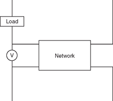
FIGURE 5-3 Relation of load, network, and voltage source.
Here is a typical broadcast application:
Entries I1 and I2 define the tag and segment number to which end 1 of the transmission line is connected. Entries I3 and I4 define the tag and segment number to which end 2 is connected.
Entry F1 specifies the characteristic impedance of the transmission line in ohms. A negative sign in front of the characteristic impedance acts as a flag for generating the transmission line with a 180-degree phase reversal (crossed line) if this is desired.
Entry F2 specifies the length of transmission line in meters. If this field is left blank, the program will use the straight line distance between the specified connection segments. If the length of the transmission line is originally specified in degrees, then it must be converted to meters with the expression
The remaining four floating-point fields are used to specify the real and imaginary parts of the shunt admittances at end 1 and end 2, respectively.
The rules for transmission line commands are the same as for network commands. All transmission line commands for a particular configuration must occur together with no other commands (except NT commands) separating them.
When the first TL or NT command is read following a command other than a TL or NT command, all previous network or transmission line data are destroyed. Hence, if a set of TL commands is to be modi-fied, all transmission line and network data must be input again in the modified form.
One or more transmission lines may be connected to any given segment. Multiple transmission lines connected to one segment are connected in parallel.
If a transmission line is connected to a segment that has been impedance loaded (i.e., through the use of an LD command), the load is placed on the segment in series with the transmission line input, similar to a network, as shown in Figure 5-3.
5.4 Network Output File Listing
If a NEC-2 run uses networks, data pertaining to those networks are listed under three categories in the output file. An excerpt from such an output file is explained as follows.
5.4.1 Network Descriptions
The network description provided by the NT commands of the NEC-2 input file is listed for confirmation under the heading - - - NETWORK DATA - - -.
Output 5-1 shows a three-tower array being driven through the antenna tuning networks. It shows the From-To listing (input/output) of the networks and the Y11, Y12, and Y22 parameters that describe the networks.
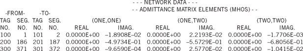
Output 5-2
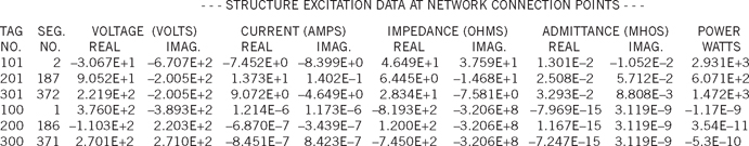
5.4.2 Source and Load Impedance to the Networks
The - - - STRUCTURE EXCITATION DATA AT NETWORK CONNECTION POINTS- - - heading in Output 5-2 lists what amounts to the source and load impedances presented to each network; that is, it shows what the network sees when looking back into the structure feeding the network, and what the network sees when looking forward into the structure the network is feeding.
In the case of ATU 1, its load is the drive point of tower 1 (wire tag 101, segment 2), listed under “IMPEDANCE(OHMS) ” as 46.49 + j37.59. Its source in this case is the very short dummy wire provided as the means to feed the network (wire tag 100, segment 1). So, looking back into the structure, the network sees −8.19 − j3.2E + 08, which is the primarily capacitive reactance of the very short wire.
ATU 2 and ATU 3 are shown in a like manner.
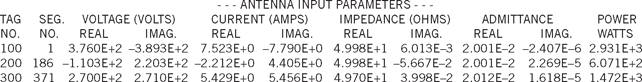
5.4.3 Network Input Parameters
The impedance seen looking into the input terminals of the network is listed in Output 5-3 under the - - - ANTENNA INPUT PARAMETERS - - - heading along with the voltage appearing across the input terminals, the current into the network, and the power taken by the network.
In the case of tower 1, the input impedance presented by the ATU is 49.98 + j0.006. The input current is 7.52 − j7.79 amps peak and the network is taking 2931 watts. Towers 2 and 3 are listed in a like manner.
5.5 Exercises
5-1. Use Listing 2-1 given in Chapter 2, Section 2.3.4 as the input file for a bnec.exe run and record the drive point impedance. Modify Listing 2-1 to add 150 pf capacity in parallel with the drive voltage and do a bnec.exe run using the modified code as the input file. Compare the resulting drive point impedance with the original.
5-2. Repeat the steps in exercise 5-1 but add 300 pf capacity instead of 150 pf.
5-3. Modify the input file created in exercise 5-2 to add a network that matches the drive point impedance to 50 ohms using a 90° T-network.