6.1 Base Drive Voltages

NEC-2 requires the broadcaster to change his starting parameters from field ratios to the voltages present at the drive point of the towers. Although there are several ways to accomplish that, this section describes a modified version of the method given by Trueman in IEEE Transactions on Broadcasting, March 1988. The process, as applied to broadcasting, is explained in the sections that follow.

First, however, a word of encouragement is in order at this point. The sections that follow present some rather laborious and boring mathematics. They develop the procedure for calculating the drive point voltages that create the target field ratios and it is important to thoroughly understand the process involved. However, software has been provided on the CD included with this book to read the NEC-2 output files and to make the necessary calculations with a minimum of human effort. Thus, you may use the software in lieu of making the detailed calculations. However, it is still worthwhile to wade through the mathematics to understand the process.

6.2 Direct and Induced Currents

Recognize that the drive voltage at the base of a tower causes a current to flow in that tower. If there are other towers nearby, then the current flowing in the driven tower will induce a current flow in those nearby towers even though the nearby towers have no drive voltage of their own. Consequently, when all towers are driven, the current flowing in a given tower is the result not only of the drive voltage at its base, but also of the current flowing in the neighboring towers. In the case of three towers,

(1)

where I₁ is the total current flow in tower 1, I₁₁ is the current flow in tower 1 due exclusively to its own excitation, I₁₂ is the induced current flow in tower 1 due to the excitation of tower 2, and I₁₃ is the induced current flow in tower 1 due to the excitation of tower 3. Similar equations can be written for towers 2, 3, and so on.

NEC-2 makes it easy to view these current components. For example, a NEC-2 simulation of such a three-tower array, with each tower having been divided into twenty segments, will have a total of sixty segments displayed in the NEC-2 output file—twenty segments on tower 1, twenty additional segments on tower 2, and another twenty segments on tower 3.

If tower 1 is driven and there is no drive on towers 2 and 3, the NEC-2 output file will show I₁₁, (which is the current distribution of tower 1) on segments 1 through 20. It will also show I₂₁, (the induced current distribution of tower 2), on segments 21 through 40. Finally, it will show I₃₁, (the induced current distribution of tower 3), on segments 41 through 60. Therefore, the NEC-2 output file will have a listing of the current distribution on all three towers, although only tower 1 is driven. For example,

■ I₁₁ is the current on tower 1 due to the drive on tower 1, and the distribution appears on segments 1 through 20.

■ I₂₁ is the current on tower 2 due to the drive on tower 1, and the distribution appears on segments 21 through 40.

■ I₃₁ is the current on tower 3 due to the drive on tower 1, and the distribution appears on segments 41 through 60.

In a like manner, if in the NEC-2 simulation, only tower 2 is driven and there is no drive on towers 1 and 3, then in the NEC-2 output file,

■ I₁₂ is the current on tower 1 due to the drive on tower 2, and the distribution appears on segments 1 through 20.

■ I₂₂ is the current on tower 2 due to the drive on tower 2, and the distribution appears on segments 21 through 40.

■ I₃₂ is the current on tower 3 due to the drive on tower 2, and the distribution appears on segments 41 through 60.

Finally, if the simulation drives only tower 3 while towers 1 and 2 are not driven, then in the NEC-2 output file,

■ I₁₃ is the current on tower 1 due to the drive on tower 3, and the distribution appears on segments 1 through 20.

■ I₂₃ is the current on tower 2 due to the drive on tower 3, and the distribution appears on segments 21 through 40.

■ I₃₃ is the current on tower 3 due to the drive on tower 3, and the distribution appears on segments 41 through 60.

Now if this three-tower simulation is written so that all three towers are driven simultaneously, then each tower will have three current components flowing—the current due to its own excitation plus the current component induced from the excitation of each of the other two towers. In that case, the NEC-2 simulation output file will list the following currents by segment:

■ I₁, which is composed of I₁₁ + I₁₂ + I₁₃, and the distribution appears on segments 1 through 20.

■ I₂, which is composed of I₂₁ + I₂₂ + I₂₃, and the distribution appears on segments 21 through 40.

■ I₃, which is composed of I₃₁ + I₃₂ + I₃₃, and the distribution appears on segments 41 through 60.

Notice that these currents are of the form described in equation (1).

6.3 Current Moments

The field radiated by a tower is proportional to the total current flowing in that tower. At the horizon

(2)

where I_i(z) is the total current flowing in tower i as a function of height and is defined by

The current on tower i is the current caused by exciting tower i plus those currents induced on tower i as a result of the drive on the companion towers.

Because the current distribution on a tower is not uniform, nor is it commonly defined, the integral within the brackets of equation (2) is not easily evaluated. To overcome this difficulty, in some calculation methods, the current distribution has been assumed to be sinusoidal, thus making the integral easily evaluated. This assumption is satisfactory for many situations but it leads to error when working with tall towers and other complex configurations.

Therefore, in the NEC-2 analysis and for purposes of the explanations in this section, rather than make this sinusoidal distribution assumption, the current distribution is approximated by dividing the tower into a number of short segments, each of which carries a current of constant amplitude whose value is defined as the current that exists at the center of that particular segment. Then with the current distribution on the tower approximated by a number of segments, each of which has a particular length and each of which carries a particular current of constant amplitude over the entire length of that segment, the integral can be approximated with satisfactory accuracy by a summation of the product of current and segment length, thus

(3)

where I_j is the current in segment j and Δ_j is the length of segment j and the product is summed over N, the total number of segments. Values for both I_j(z) and Δ_jcan be obtained from the NEC-2 output file under the heading CURRENTS AND LOCATION.

Recall that the current moment is defined as the product of the current flowing in a particular segment multiplied by the length of that segment and because the current has a phase relative to some reference, the current moment is a complex number.

The term on the right side of equation (3) is seen to be the current moment of the tower furnishing the data and its value is easily obtainable from the NEC-2 output file. Stating this in general terms gives

(4)

where C_i is the total current moment of tower i, N_i is the number of segments on tower i, Δ_ij is the length of segment j on tower i, and I_ij is the current on segment j of tower i.

To accommodate the case where Δ_ij is not vertical, then the factor sin α_ijis added within the summation where α_ij is alpha, the vertical angle of Δ_ij, as read from the NEC-2 output file. Equation 4 then becomes

(5)

6.4 Development Concept

The task now is to describe a method that can be implemented in a postprocessing computer program to convert the desired field ratios to a set of base drive voltages that will generate those field ratios.

From Section 6.2, we see that we can determine the current distribution of the various components of current flowing in each tower by individually driving each tower while the companion towers are left with no drive. Then Section 6.3 shows how the current moments are calculated from those current distributions. This section uses a three-tower array to explain a special utilization of those procedures to determine the desired base drive voltages.

To generate the data for this analysis, it is necessary to make three NEC-2 runs with an input file and an output file for each run. The first NEC-2 run calls for driving each tower individually with 1 + j0 volt while the companion tower bases are shorted to ground to ensure zero volts at each base. Next, we make a second NEC-2 run using a set of normalized drive voltages that have been determined from the results of the first run. The normalized drive voltages generate the correct pattern shape but not the correct pattern size. Finally, to create the correct pattern size, a third NEC-2 run is made using final drive voltages, which are obtained by scaling the normalized voltages to the full power level.

To keep track of the several files, it is helpful to be consistent in naming them. In this work, the files associated with the unity excitation have been named CALL_1.NEC and CALL_1.OUT to identify the NEC-2 input file and the corresponding output file. The NEC-2 runs using the normalized drive voltages are named CALL_N.NEC and CALL_N.OUT and the files for the final run are named simply CALL.NEC and CALL.OUT

6.4.1 Unity Drive

The first step is to characterize the array. This is done by individually driving each tower of the array with 1.0 + j0.0 volt while the companion towers are grounded. The tower currents as described in Section 6.2 will be obtained as a result of this unity drive and the related current moments can then be determined as described in Section 6.3.

Excitation to the driven tower is placed on the base insulator segment and the other towers are grounded by giving them no excitation.

It is not necessary to run NEC-2 three times to create the three current files necessary to calculate the unity drive current moments. This can be done in a single NEC-2 run by repeating the drive commands. For example, including these NEC-2 commands

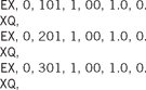
in the CALL_1.NEC file will place the 1.0 + j0 volt drive on tower 1 with the companion towers grounded, then execute a NEC-2 analysis. Following that, it will place the 1.0 + j0 drive on tower 2 with the companion towers grounded, then execute another NEC-2 analysis. Finally, the commands will place the 1.0 + j0 drive on tower 3 with the companion towers grounded and execute yet another NEC-2 analysis. Each NEC-2 execution will generate the corresponding current listings in the output file for each excitation command.

6.4.2 Normalized Drive

Since the towers of the three-tower array were driven with 1.0 + j0 volt, the current moments calculated from the resulting current sets will be the current moment per volt with units of ampere-meter per volt (A-M/V). Thus, to obtain the current moment for any other drive voltage on the tower, the current moment per volt can be multiplied by the applied volts, which may be, and in this case is, a complex number. For example, with a drive voltage of V₁ on tower 1,

In a like manner, if tower 2 is driven with V₂ volts and towers 1 and 3 shorted, the resulting current moments will be

Also, driving tower 3 with V₃ and towers 1 and 2 shorted gives

Finally, if all three tower s are dr iven simultaneously with V₁, V₂, and V₃, then each induces a current in the others with the resulting total current moments being

(5)

(6)

(7)

Stated in general terms,

Since the field is directly proportional to the current moment, then the field ratio is

where C_k is the current moment of the reference tower. If we select tower 1 to be the reference tower, then

At this point, this development deviates from that of Trueman to take a less rigorous but somewhat more convenient path.

Dividing equations (5), (6), and (7) by the current moment of the reference tower, C_k, and recognizing that C_i/C_k = F_i results in

(8)

(9)

(10)

where the left side of the equations can be the desired field ratios, in which case the primed Vs represent the base drive voltages normalized to the current moment of the reference tower. The normalized drive voltages have the units of volts per ampere-meter.

We now reason that there exists a set of complex voltages for V₁^′ V₂^′, and V₃^′ that will operate on the set of current moments to yield the desired field ratios. We have values for all the variables except the three normalized drive voltages, therefore we have a set of simultaneous equations consisting of three equations with three unknowns. We can now solve for those unknown normalized drive voltages, taking due notice that all variables are complex.

The result thus obtained is not the final answer, however. Because the drive voltages have been normalized to the reference current moment, they will create the desired pattern shape but they will not create the correct pattern size.

6.4.3 Full Power Drive

To get the correct pattern size, we must do a NEC-2 run using the normalized drive voltages. It is suggested that these input and output files be named CALL_N.NEC and CALL_N.OUT, respectively. Review the output file thus obtained (CALL_N.OUT) and take note of the total input power listed under the heading — POWER BUDGET-. Call this value P_nand call the desired full power P_f. Then, to obtain the full power drive voltages, we must scale the normalized drive voltages by the factor

(11)

Finally, a third NEC-2 run can be made (naming input and output files CALL.NEC and CALL.OUT) using the scaled full power drive voltages to obtain the correct pattern size and power level.

6.4.4 Shunt Reactance and Networks

It is important to know that if the tower model includes a reactance in parallel with the exciting voltage, such as might be implemented using the network configuration described in Figure 5-2(c), then that reactance may be in place on the excited tower when the individual towers are excited with 1.0 + j0.0 volts, as described in Section 6.4.1. However, be aware that while an individual tower is being excited, the remaining towers of the array must be grounded. Therefore, any reactance that appears in series with the tower must not be in place on towers that are to be grounded. In short, the NT command should be paired with the corresponding EX command in defining the excitation, as opposed to leaving all NT commands in place during the individual excitations.

Of course, the shunting reactance should be in its proper place throughout the remaining steps of the excitation voltage calculation.

Moreover, if the tower model includes both a shunt reactance and a series reactance, be careful about using the network described in Figure 5-2(d). The transfer function of that network varies with the terminating impedance; thus, it is not possible to accurately transfer the base drive voltage from the tower base to the input of the network. The work-around for this is to use the network configuration in Figure 5-2(c) to simulate the shunt reactance while calculating the base drive voltages. Once the drive point impedances have been determined, simply mentally add the series reactance to the calculated drive point impedance.

6.5 Example: A Three-Tower Array

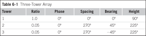
The procedure for calculating the driving point voltage will be summarized with a simple three-tower example using a transmitter operating on 1500 kHz with 5000 watts and seeking the array parameters shown in Table 6-1.

This example was chosen to demonstrate that the procedure can accommodate various conditions including tall towers and towers of different heights as well as widely differing field ratios.

6.5.1 Create a Unity Drive File

The first task in determining base drive voltages is to generate a NEC-2 input file that will drive each of the towers individually and sequentially with 1.0 + j0.0 while the companion towers are grounded. Listing 6-1 defines the geometry of the array, installs the operating parameters, and drives each tower in sequence. Notice particularly how the EX commands are listed and executed individually.

Listing 6-1

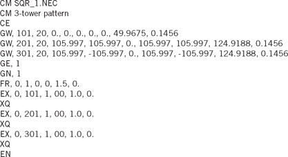
You are encouraged to run this input file and create an output file named SQR_1.OUT. Refer to your output file for the following discussion.

6.5.2 Calculate Unity Drive Current Moments

The unity drive current moments are used in conjunction with equations (8), (9), and (10) to calculate the normalized drive voltage. For this three-tower array, three current moments are calculated for each of the three towers.

Tower 1 Moments

The SQR_1.OUT output file will contain three sets of current listings. The first listing will be under the heading — CURRENTS AND LOCATIONS — and will follow the listing of the first EX card, which shows that tower 1 is the driven tower. That current listing contains the current distribution on each of the three towers as a result of driving tower 1.

Segments 1 through 20 show I₁₁, which is the current on tower 1 due to its own drive. Segments 21 through 40 show I₂₁, which is the current on tower 2 due to the drive on tower 1, and segments 41 through 60 show I₃₁, which is the current on tower 3 due to the drive on tower 1.

The current moment components C₁₁, C₂₁, and C₃₁ of equations (5), (6), and (7) can be computed from these current distributions by noting that the — CURRENTS AND LOCATIONS — listing shows the length of each segment in addition to the current on each segment. These can be applied to equation (4) to determine the current moment; for example,

(11)

where j represents the segment number, in this instance running from 1 to 20 on tower 1.

In this example, notice that the segment length is constant on each tower, so it was factored out of the summation as a multiplier. Also notice that all segments are vertical, so the factor sin α. is not required. Do not overlook the fact that in the output file, the segment length is given in units of wavelength. This must be converted to meters by multiplying the listing by the wavelength. In the instance of tower 1, the segment length is 0.0125 × 199.87 meters = 2.498 meters. Thus, equation (11) becomes

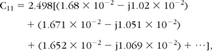
(12)

with the result that C₁₁ = (0.55278 –j0.38736)

The current is taken in the real/imaginary form rather than the polar form to facilitate the addition.

In a like manner, C₂₁ and C₃₁ can be determined from the remainder of the current listing using

(13)

where the segments on tower 2 run from 21 through 40 with the segment length = 0.03125 λ, or 6.246 meters, resulting in

And finally,

(14)

where the segments on tower 3 run from 41 through 60 with segment length = 0.03125λ, or 6.246 meters, so

Tower 2 Moments

Next, following the listing of the EX command, driving tower 2 will be the set of current listings resulting from the drive on tower 2. It, too, will be under a heading — CURRENTS AND LOCATIONS —. Again, segments 1 through 20 show the current distribution on tower 1 due to the drive on tower 2, segments 21 through 40 show the current on tower 2 due to its own drive, and segments 41 through 60 show the current on tower 3 due to the drive on tower 2.

The current moment components C₁₂ C₂₂, and C₃₂ of equations (5), (6), and (7) can be computed from these current distributions by following the same procedure described previously and again noting that in the instance of towers 2 and 3, the segment length is 0.03125 × 19987 meters = 6.246 meters.

(15)

so

Also

(16)

then

Finally,

(17)

and

Tower 3 Moments

Following the listing of the EX command driving tower 3 will be the third set of current listings. It too will be under the heading — CURRENTS AND LOCATIONS —. Segments 1 through 20 show the current distribution on tower 1 due to the drive on tower 3, segments 21 through 40 show the current on tower 2 due to the drive on tower 3, and segments 41 through 60 show the current on tower 3 due to its own drive.

In a manner similar to that above, the current moment components C₁₃, C₂₃, and C₃₃ of equations (5), (6), and (7) can be computed from these current distributions by following the same procedure described previously.

(18)

results in

Also

(19)

so

Finally,

(20)

and

6.5.3 Solve for the Normalized Drive Voltages

The current moments just calculated can be placed in equations (8), (9), and (10). Then both sides of the equations are divided by the current moment of the reference tower (C₁). Since C_i/C₁ = F_i, we can replace the left side of equations (8), (9), and (10) with the desired field ratios. The results are:

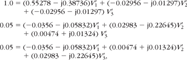
where the V′ values are the drive voltages normalized to the reference current moment.

These three equations leave only the values for the three normalized drive voltages as unknowns, so they can be solved as a set of simultaneous equations.

A small postprocessing computer program has been written to read the SQR_1.OUT file and calculate the current moments thus generated. Thereafter, it solves the N equations in N unknowns to obtain the normalized drive voltages. The program NECDRV2.EXE performs that function and is included on the CD included with this book.

In this instance, using the parameters given earlier and running NECDRV2.EXE yields the following results for the normalized drive voltages:

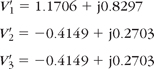
These normalized drive voltages are now used to drive the three towers simultaneously by placing these drive voltages in a SQR_N.NEC

Listing 6-1(a)

Listing 6-1(b)

file. This is most conveniently done by copying the SQR_1.NEC file to SQR_N.NEC and modifying the EX commands to read as shown in Listing 6-1(a).

Once created, the SQR_N.NEC file is run using bnec.exe to generate the SQR_N.OUT file.

6.5.4 Determine the Full Power Drive Voltage

The SQR_N.OUT file shows the correct drive point impedances and other parameters but it does not create the correct power level, nor would it create the correct pattern size. This is corrected by scaling the normalized drive voltages by the square root of the ratio of desired power to the normalized power.

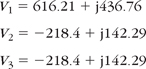
Under the heading — POWER BUDGET —, the SQR_N.OUT file shows a total normalized power of 1.8044E-02 watts. The scale factor to get this up to 5000 watts is

The full power drive voltages are obtained by multiplying the normalized drive voltages by the factor 526.40. Thus,

The SQR_N.NEC normalized input file is copied to SQR.NEC, and SQR.NEC is edited to replace the normalized voltages on the EX commands with the full power drive voltages, as shown in Listing 6-1(b).

Running SQR.NEC generates SQR.OUT, which is the full power output file that is usually created in a normal NEC-2 design analysis. SQR. OUT contains all the information necessary for the usual array design and is where the design effort would normally stop.

6.6 Exercises

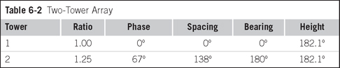
Consider a two-tower array having the parameters shown in Table 6-2. The transmitter operates on 870 kHz with a power of 50,000 watts. The towers are identical. Use the tower model shown in Figure 3-1(c) with twenty segments. The drive wire is the length of one segment with a radius equal to 6 inches. The remainder of the radiator is a triangular tower having a face width of 48 inches.

6-1. Give NEC-2 calculated values for the following:

(a) Drive point impedance of each tower

(b) Power to be delivered to each tower.

(c) Expected antenna monitor reading if tower currents are sampled with current transformers located at the output of the antenna-tuning network

(d) At what height on the towers should a sampling loop be mounted so that the antenna monitor readings will closely approximate the far-field ratios?

6-2. Repeat exercise 6–1 with 250 pf shunting the drive voltages.

(a) What effect does the shunting capacity have on the drive point impedance? Why?

(b) What effect does the shunting capacity have on the power required by each tower. Why?

(c) Does the shunting capacity affect the antenna monitor readings?

(d) What characteristic of this array suggests that it is sensitive to the capacity shunting the drive voltage?

(e) What is a likely source of this shunting capacity?