

7.1 Overview
NEC-2 output reports are quite voluminous and have long lines that make them difficult to read and difficult to print. A convenient way to view them is to open the file in WordPad using the command “Wordpad CALL.OUT”. To conveniently print a hard copy of the file, select the entire file and reduce the font to size 6 so the long lines will fit on 8½ × 11 paper in the portrait orientation. A larger font can be used to print it in the landscape orientation.
Not all of the output report is necessary for the usual broadcast work. For example, the segmentation data adds considerably to the volume of the report and contributes very little in usual broadcast work. Also, the far-field pattern listing adds more that 361 lines to the report but they are used only to plot the pattern. Therefore, one might want to create a condensed output file by copying the CALL.OUT file to CALL_C.OUT and from the latter, delete unwanted portions to generate a smaller working file. In any event, the original CALL.OUT file should be retained so the entire file is available for future reference.
For an even more concise output report, a simple computer program can be written to read the CALL.OUT file and print pertinent information such as drive point impedance, power budget, and base currents.
The NEC-2 output file is a source of much information that is not listed directly in the file. With a little manipulation of the output file content, the additional information can be retrieved to yield a deeper insight. Simple computer programs may be written to read the NEC-2 output file directly and then process the data as desired. It is beyond the scope of this book to cover programming methods to accomplish this, but the necessary methods are well known to those who are knowledgeable in computer programming. The sections that follow describe the concepts embodied in those computer programs and provide some examples.
7.2 Verify the Field Ratios
Once the base drive voltages have been computed and used to render a NEC-2 output file, it is very reassuring to know that the voltages as calculated do, in fact, create the desired field ratios.
The NEC-2 output file contains the current distribution listing that resulted from the actual drive voltages used to create that file. As explained earlier, the current moments can be calculated from these current distributions and the field ratios can then be determined from those current moments. In the case of the example file SQR_N.OUT created in Chapter 6, the current moments are
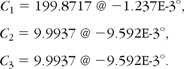
Recalling that Fi = Ci/Ck, we can write
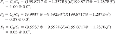
which agree perfectly with the desired field ratios listed in the example.
7.3 Plot Far-Field Radiation Pattern
The RP command creates a listing of the radiation pattern in the output file. Once this listing is made, a postprocessing program can be written to read the output file and plot the resulting pattern. If the vertical angle (θ) is held constant while the azimuth angle (Φ) is varied, the horizontal pattern is generated. An example of such a plot is shown in Figure 7-1 where the data is taken from the file SQR.OUT as created in Chapter 6.
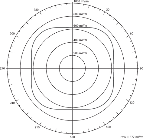
FIGURE 7-1![]()
Radiation pattern of SQR.OUT.
If Φ is held constant while θ is varied, then the vertical pattern is generated.
As an alternative, the PL command may be used to generate a separate data file to hold only the radiation pattern data. A typical PL command is
The command will generate a table of values that can be adapted to any available plotting routine. Refer to the PL command in Appendix A for additional details.
7.4 Detuning Unused Towers
When it is desirable to create a circular radiation pattern by restricting all radiation to a single tower of a multiple tower array, two approaches are possible and both can be simulated by a NEC-2 analysis. The first approach is to handle the generation of the circular pattern as one might handle any other pattern; that is, calculate the drive voltages that yield a field ratio of 1 @ 0° for the driven tower and 0 @ 0° for all unused towers. This creates a perfectly circular pattern and is an excellent analysis tool. Unfortunately, the method suffers the disadvantage of requiring the expense of a complete power dividing and phasing capability to physically implement such arrangement.
The second approach is much less expensive and therefore is the most often used. Recall that the driven tower induces a current flow in the unused towers of an array and that the induced current flow radiates a field that causes the distortion of the desired nondirectional pattern. The radiated field caused by the induced current is expressed mathematically as
where I(z) is the induced current as a function of height and the integral in the expression is the current moment of the unused tower. It is clear, then, that if the current moment can be made to be 0 (or near 0), then the radiated field from the unused tower is also made to be 0 (or near 0). That is the principle upon which the concept of detuning an unused tower is based.
There are several options available to accomplish the task. The first option, and perhaps the least expensive, is to simply open the base of the unused towers, thus reducing the current moment by reducing the current flow. This is usually satisfactory for short towers but the taller towers require a bit more attention to nullify the effect of the current that continues to flow even when the tower base is opened. In that case, base loading may be used to reduce the current moment created by the induced current.
7.4.1 Detuning by Base Loading
The process of base loading an unused tower to reduce its parasitic radiation includes grounding the tower base through an inductance whose value has been selected so as to create a current distribution on the tower that minimizes the current moment. A good starting value for the base load inductance can be obtained by making a NEC-2 analysis in which all towers are driven to create a field ratio of 1.0 @ 0° for the nondirectional tower and 0.0 @ 0° for each unused tower.
From the output file generated by that analysis, the drive point impedance of each unused tower is examined and the conjugate of the reactive component is taken as a good estimate of the base loading reactance necessary to detune that unused tower. The conjugate reactance is called a good estimate because some adjustment to that value may be necessary if the resistive component of the unused tower's drive point impedance is large. Therefore, the value of the base loading reactance should be verified by iterating larger and smaller values. If more than one unused tower is involved, then using the average value of inductance in all unused towers will usually be effective if the towers are identical.
The appropriate value of inductance can also be determined entirely by an iteration process, that is, by arbitrarily selecting a starting value for the base load inductance (perhaps 10 to 50 μH) then running a NEC-2 simulation to calculate the resulting current moments for the towers of interest. That process is then repeated with changing inductance values until the value of inductance is found that reduces the current moments sufficiently to produce a satisfactory circular radiation pattern from the driven tower.
Example: Detuning by Base Loading
This example describes the detuning of seven of the eight towers in an array configured in two rows of four towers each. Each tower is 203° in height and the spacing between towers is in the order of 100°. Tower 7 is fed with 1000 watts while the other towers are detuned in an effort to create a circular pattern.
Taller towers exhibit a different behavior than do shorter towers. Shorter towers cause the most severe pattern distortion when the unused towers are connected to ground. In this example using taller towers, the most severe pattern distortion occurs when the unused towers are left open.
See Figure 7-2 for the pattern obtained when the bases are left open and Figure 7-3 for the pattern obtained when the bases are shorted directly to ground.
Both patterns fail to meet the requirement for a circular pattern, so it is mandatory that some means be used to improve the circularity. To determine the base loading inductance, a NEC-2 analysis was run to determine the drive voltages necessary to create a field ratio of 1 @ 0° for tower 7 and 0 @ 0° for the companion towers. The output file for this analysis was studied to confirm the circularity of the pattern and also to determine the drive point impedance of each companion tower. From the drive point impedances, the conjugate of the reactive part was taken as the reactance for base loading. For the eight-tower array being considered, the conjugate reactances ranged from + j118 to + j136, corresponding to inductances within the range 13.62 μH to 15.54 μH. A base loading inductance of 15 μH was selected for each of the companion towers.
A NEC-2 simulation was run with the base of the unused towers connected to ground through the 15 μH inductor. The resulting NEC-2 output file was processed to calculate the field ratios that resulted from the induced current in each tower, and those field ratios were summed as a figure of merit. The value of inductance was iterated and the field
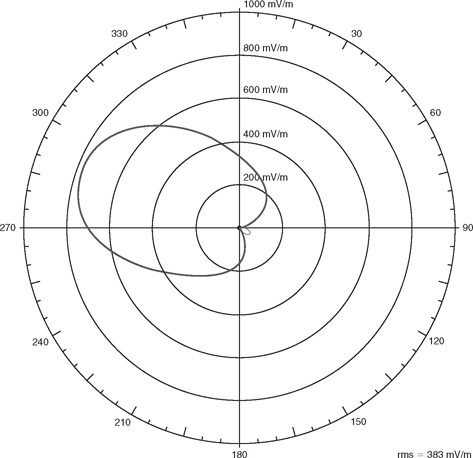
FIGURE 7-2![]()
Nondirectional pattern of an eight-tower array with the unused towers open.
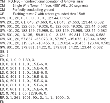
ratios were calculated and their magnitude summed for each value of inductance. The 15 μH inductor was verified as that value that produced the smallest field ratio sum. The calculated field ratios were:
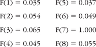
The minimum field ratio sum was 0.3389.
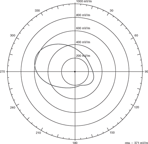
FIGURE 7-3![]()
Nondirectional pattern of an eight-tower array with the unused towers grounded.
The resulting radiation pattern is shown in Figure 7-4. While the result is less than ideal, it is indeed an improvement over that obtained by simply grounding the bases or leaving them open. An attempt was made to further reduce the field ratios by using the base loading inductance individually calculated for each unused tower, but the reduction was not significant.
Base Loading Input File Listing
The following NEC-2 input file (Listing 7.1 on page 90) generates the radiation pattern shown in Figure 7-4. The LD commands provide the base loading.
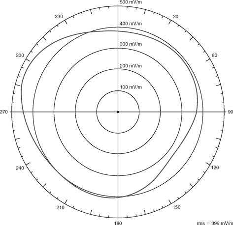
FIGURE 7-4 Nondirectional pattern of an eight-tower array using base loading.
7.4.2 Detuning by Skirting
The previous example demonstrates that tall towers do not respond well to detuning by base loading. Somewhat better results can be obtained by using a 90° skirt at the top of the tower to create the effect of a shorter tower. The example that follows demonstrates that concept.
Example: Detuning by Skirting
The array used in the previous example will be used in this example to demonstrate the increased effectiveness of detuning by using a skirt
on a tall tower. For convenience, a four-wire skirt is used with the top end connected to the top of the tower. The skirt extends 90° from the top of the tower and its lower end effectively terminates the tower in a high impedance at the lower end of the skirt. The 203° skirted tower now behaves as though it were a simple 113° tower, and thus it can be detuned effectively by simply leaving its base open.
The details of creating the skirt are described in Chapter 9, Top Loaded and Skirted Towers. For now it is sufficient to explain that the tower with skirt wires was modeled as tower 1. then the GM command was used to copy the entire skirted tower to the locations of towers 2 through 6 and again at the location of tower 8. Tower 7 was not skirted because it is the driven tower in the nondirectional mode. The viewing program, NVCOMP.EXE, was used to verify the correctness of the total array. Figure 7-5 shows the NVCOMP.EXE display of the array. Tower 1 is the rightmost tower on the back row with tower 5 being in front of tower 1.
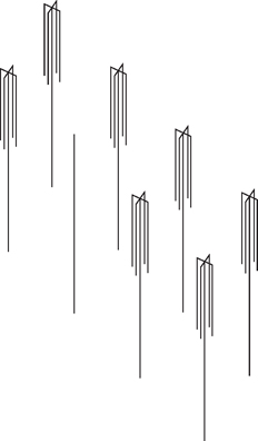
FIGURE 7-5![]()
NVCOMP.EXE display of eight-tower array detuned with top skirts.
It is worthwhile to note here that from a practical standpoint, a system such as this can be implemented by using a contactor to connect the lower end of the skirt to the tower when the array is in the directional mode. The contactors will be open in the nondirectional mode.
With the skirts in place and the tower bases open, the calculated field ratios are:
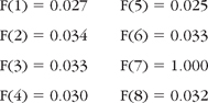
The minimum field ratio sum is 0.2140.
These values are somewhat smaller than those given in the Example: Detuning by Base Loading section when base loading was used. The resulting radiation pattern is shown in Figure 7-6 and is indeed an improvement over that shown in Figure 7-4.
In an attempt to improve the circularity even more by combining the skirted method with base loading, the tower bases were connected to ground through selected values of inductance. The smallest field ratio sum was obtained with an inductance of 47 μH in each base and the field ratio sum decreased significantly to 0.0220. Surprisingly, however, the circularity of the radiation pattern showed no practical improvement. Where the pattern in Figure 7-6 shows a compression at 270°, the revised pattern showed an equivalent bulge at 110°. The improvement did not appear to warrant the change.
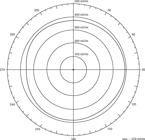
FIGURE 7-6![]()
Nondirectional pattern of eight-tower array using skirt detuning.
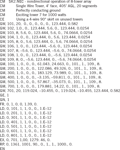
Input File Listing: Detune by Skirting
Listing 7-2 is the NEC-2 input file that yields the pattern of Figure 7-6.
The LD commands in Listing 7-2 insert a 1 pF capacitor in the bottom segment of the unused towers to create the open base. The GW, 100 series commands create tower 1 and its skirt. The GM commands copy the complete tower 1 to the locations of the other unused towers. The command GW, 701, is tower 7. It is not skirted and it is driven by the EX command.
Listing 7-2
7.5 Antenna Monitor Readings
Perhaps the most useful information furnished by the NEC-2 output file is a prediction of the antenna monitor readings that will exist when the array is properly adjusted. This is especially important during the initial adjustment of a new array employing towers with heights greater than 90°.
By sampling the currents on each tower of the array the antenna monitor gives a comparative indication of the magnitude ratio and phase of the tower current relative to that of the reference tower. Once properly set up, the antenna monitor oversees and provides visibility into the operation of the directional antenna.
When adjusting a new array without a NEC-2 analysis, however, the relationship between the radiated far fields and the antenna monitor readings are not yet established. Therefore, it is necessary to employ a cadre of field technicians, each stationed at a measuring point and equipped with a field strength meter and two-way radio, to “talk” the radiation pattern into spec compliance as the engineer makes adjustments on the phasing equipment in the transmitter building. When the array meets its pattern requirements, the antenna monitor readings (whatever they might be) are logged and become the onsite indicator of the array's proper performance.
Fortunately, the amount of field work and adjustment time can be greatly reduced by using information gained from a NEC-2 analysis. Because the amplitude and phase of the current on a tower are not constant from bottom to top, the height on the tower at which the current is sampled will determine the ratio and phase indication on the antenna monitor. If, on each tower, the antenna monitor sample is taken at that height on the tower where the ratio and phase of the tower current match the target field ratio and phase, then the antenna monitor will give indications closely approximating the radiated field ratios. That being the case, then during the adjustment process, once the monitor readings match the target values (regardless of how they are achieved), the pattern will very nearly coincide with the target pattern. Only a minimum amount of field work will then be required to verify the pattern and to make adjustments as might be caused by parasitic radiations or other causes.
7.5.1 Optimum Height for Sample Loops
Refer to the heading — CURRENTS AND LOCATIONS — in the NEC-2 output file SQR.OUT, as created in Chapter 6. Remember that the target field ratio phase for towers 1, 2, and 3 are 0° 0°, and 0°, respectively. Also, remember that segments 1 through 20 are located on tower 1, segments 21 through 41 are located on tower 2, and segments 41 through 60 are on tower 3. We can determine the optimum height for the sample loops by finding the height on each tower where the phase of the tower current goes through the corresponding field ratio phase, which, in this example, is 0° for each tower.
A portion of the current distribution listing is shown in Output 7-1.
Output 7-1
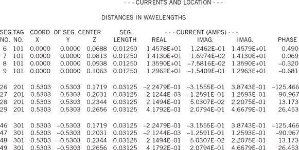
Notice that within segments 1 through 20 (tower 1), the phase of the current goes through 0 between segments 7 and 8. We could interpolate between these segments for an exact height but for all practical purposes we can say that the phase is 0 at the center of segment 7 because at that height the phase is only +0.069°. The height of the center of segment 7 is given by the table as 0.0813 λ = 16.25 meters, or 53.31 feet. Thus on tower 1 the sample loop should be mounted at a height of approximately 53 feet 4 inches to give an antenna monitor indication representative of the field ratio.
In the case of tower 2, which contains segments 21 through 40, the phase of the current goes through 0° between segments 27 and 28. But notice here that the phase changes radically from −91° on segment 27 to +13° on segment 28. Therefore, it is imperative that the correct height be determined by interpolating between the two segments. Carrying out an interpolation shows that the current goes through 0° at 0.2304 λ. Thus the desired height for the current sample loop on tower 2 is 0.2304 λ = 46.05 meters, or 151 feet, 1.0 inch.
Tower 3 is the same height as tower 2 and seeks the same phase, so the results are the same as those for tower 2. The sample loop on tower 3 should be mounted at a height of 151 feet, 1 inch.
If all three towers were of the same height, then the analysis would lead to mounting the sample loops at the same height on each tower, regardless of the phase of each field ratio.
The interpolation may be carried out on the current magnitudes in addition to the phase. However, a word of caution is in order. With small field ratios, the round-off error and other uncertainties inherent in NEC-2 may yield significant error in the second and greater decimal place. For that reason, it is recommended that the sample loop be positioned based on phase and not magnitude.
7.5.2 Arbitrary Height for Sample Loops
There are occasions when existing sample loops must be used, or perhaps it is desired to forego an interpolation, in which case the antenna monitor indications for the correctly adjusted array can be predicted even though the samples are taken at an arbitrary height.
If, in this example, the sample loops were arbitrarily mounted at the same height on each tower, then the antenna monitor readings would
be quite different from the field ratios, but they would still be usable when initially adjusting the array.
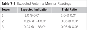
Consider mounting the sample loops at a height of 133 feet on each of the three towers. On tower 1 this height is segment 17, where the current is 5.21A @ −2.97°. On towers 2 and 3 this height is segment 27 and 47, respectively, where the current is 1.26A @ −90.97° on both towers. The antenna monitor gives readings normalized to the reference tower (1 in this case) so to correctly set up the array, the network components should be adjusted such that the antenna monitor reads as shown in Table 7-1.
This is very useful information because the monitor indications are so different from the field ratio. It is unlikely that one would have anticipated their value during the tune-up process. The NEC-2 analysis thus eliminates a considerable amount of trial and error during the adjustment process.
7.5.3 Base Current Samples
Should the designer of this array elect to monitor the base current using current transformers located at the output of the antenna matching network, the expected monitor readings for the correctly adjusted array can be anticipated by noting the current at the feed points, as shown in the SQR.OUT file, a partial listing of which appears in Table 7-2.
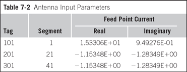
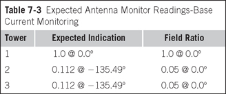
Where tag 101, segment 1 is the feed point to tower 1; tag 201, segment 21 is the feed to tower 2; and tag 301, segment 41 is the feed to tower 3. The expected monitor readings are obtained by normalizing the base currents listed in Table 7-2 to the current going to tower 1; the monitor readings to be expected when the array is properly adjusted are given in Table 7-3.
Again the NEC-2 analysis is very beneficial because the expected monitor readings are substantially different from the target field ratios.
Another word of caution is in order at this point. Shunt reactance across the drive point will alter the drive point impedance and thus the drive point current. The drive point current shown under the heading “Antenna Input Parameters” is the result of the applied voltage and the effect of the tower impedance as paralleled by any shunt reactance that has been included in the model. Thus the current listed for a given tag and segment under the heading — ANTENNA INPUT PARAMETERS — is the sum of the tower current and the current through the modeled shunt reactance. At the same time, the current listed under the — CURRENTS AND LOCATION — heading for the same tag and segment combination reflects only the tower current and does not include the current through the modeled shunt reactance.
Thus, when predicting the antenna monitor readings created from samples of the base current taken at the output of the tuning unit, one must read the appropriate tag and segment currents under the heading — ANTENNA INPUT PARAMETERS — as opposed to the currents listed under the heading — CURRENTS AND LOCATIONS — even though the tag and segment numbers are the same at both listings.
Moreover, if the NEC-2 model does not accurately duplicate the actual physical shunting reactance, then the currents predicted by the
NEC-2 analysis will not be consistent with the actual currents and the predicted monitor readings based on the drive point currents will be in error.
Notwithstanding modeling by measurement, it is not likely that one will be able to accurately duplicate the actual physical shunting reactance when modeling an array. Therefore, basing the initial antenna monitor readings on the base current ratios is not as accurate as basing them on the base voltage ratios or on current samples taken from monitor loops mounted on the tower.
Once the array has been adjusted to meet the specifications, however, then the base drive current samples are an excellent reference to monitor for any changes that might affect the array's operation.
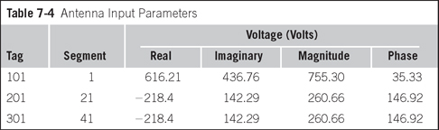
7.5.4 Base Voltage Samples
If it is preferable not to use tower-mounted current sampling loops; the base voltage ratios are the better choice of base parameters to use for determining the initial antenna monitor readings. The base voltage determines the current distribution on the tower; thus, it must be set to the correct value regardless of shunt reactance. The NEC-2 analysis defines the voltage ratios; thus, it provides an excellent indication of the predicted monitor readings when the monitor inputs are voltage samples.
For this example, the base voltages are read from the output file, as shown in Table 7-4. The voltages shown in the table, normalized to tower 1, give the expected monitor readings shown in Table 7-5.
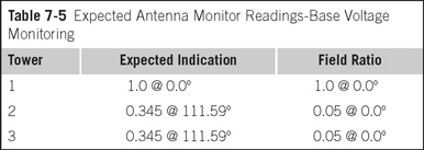
Again, it is not likely that one would have anticipated these monitor readings during the tune-up process. The NEC-2 analysis thus eliminates a considerable amount of trial and error during the adjustment process.
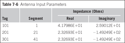
7.6 Drive Point Impedance
The drive point impedances are listed in the SQR.OUT file under — ANTENNA INPUT PARMETERS —, as shown in the partial listing of Table 7-6.
Thus the calculated drive point impedances are:
| Tower | Impedance |
| 1 | 41.8 + j25.9 |
| 2 | 23.3 − j149.2 |
| 3 | 23.3 − j149.2 |
7.6.1 Drive Point Impedance When Using a Network
Consider now the instance where matching networks are used to transform each of the above impedances to 50 + j0. To do that, the SQR.NEC file is copied and renamed NET.NEC and modified to add the networks.
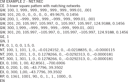
For each network we must add a dummy wire to which we connect the input of that network. These dummy wires are tag 100, tag 200, and tag 300 in Listing 7-3. Notice that the dummy wires are located far away and are very short to minimize the effect they might have on the array radiation.
The output of the networks are connected to the base of each tower on the segment where the original drive voltage had been placed.
The matching networks are designed using the usual T-network procedures. The network Y-parameters are then calculated as described in Section 5.2.1 and the NT commands are added to the input file.
In this particular case, the complex base impedances were transformed to 50 Ω resistive with an arbitrary +90° phase shift. The base drive voltages, which have been calculated to give the desired pattern, are translated from the tower base to the input of the matching networks by recalling that the phase shift within the network refers to current phase shift not voltage phase shift. The modified input file is as shown in Listing 7-3.
Run Listing 7-3 and name the output file NET.OUT, then the network parameters are listed in the NET.OUT output file under the heading — NETWORK DATA —, as shown in the partial listing of Output 7-2.
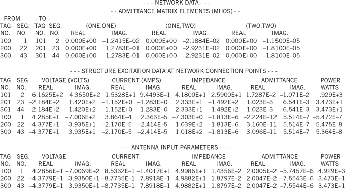
The voltage at the tower base is shown as the network output voltage at tags 101, 201, and 301 under the heading — STRUCTURE EXCITATION DATA AT NETWORK CONNECTION POINTS — in the NET.OUT output file. Under the same heading, the voltage at the input to the matching network is shown at tag 100, tag 200, and tag 300.
Finally, the results of the impedance transformation is shown under the heading — ANTENNA INPUT PARAMETERS — where the input impedance is shown as 49.99 + j0.01 for tower 1 and 49.88 + j0.02 for towers 2 and 3.
7.7 Exercises
7.1. Modify Listing 7-2 shown in Section 7.4.2 to convert the array to the directional mode by adding a spider connecting the bottom end of the skirts to the towers. Confirm the change by viewing the results with NVCOMP.EXE.
7.2. Create a NEC-2 input file by further modifying Listing 7-2 to change the drive voltage from the nondirectional mode to the directional mode using drive voltages as follows:
| Tower | Voltage |
| 1 | −191.38 + j475.31 |
| 2 | −851.97 − j573.01 |
| 3 | 1594.97 + j426.46 |
| 4 | −780.83 + j1439.34 |
| 5 | − 935.25 − j48.85 |
| 6 | 854.38 − j1604.54 |
| 7 | − 167.64 − j2163.19 |
| 8 | − 1564.52 − j1330.29 |
Do a bnec.exe run using the modified input file and confirm that the power to the array is 5000 watts.
7-3. If the monitor system uses current transformers to monitor the tower feed point currents, what will be the antenna monitor indications when using tower 3 as the reference tower?
7-4. Use the tower feed point voltages to determine the expected antenna monitor readings when the array is adjusted correctly. Compare those results with those obtained when monitoring the base currents in exercise 7-3. Which is most reliable? Why?