Notice

The input commands listed in this appendix have been taken from Naval Ocean Systems Center Technical Document 116 (TD 116), volume 2, Numerical Electromagnetic Code (NEC) — Method of Moments, Part III: User's Guide, revised 2 January 1980.

Contents

1.0  Comment Commands (CM, CE)

1.1  Comment (CM, CE) 188

2.0  Structure Geometry Commands

2.1  Wire Arc Specification (GA) 190

2.2  End Geometry Input (GE) 191

2.3  Read NGF File (GF) 193

2.4  Helix and Spiral Specification (GH) 194

2.5  Coordinate Transformation (GM) 195

2.6  Geometry Print Control (GP) 197

2.7  Generate Cylindrical Structure (GR) 198

2.8  Scale Structure Dimensions (GS) 201

2.9  Wire Specification (GW, GC) 202

2.10  Reflection in Coordinate Planes (GX) 205

2.11  Surface Patch (SP) 208

2.12  Multiple Patch Surface (SM) 210

3.0  Program Control Commands

3.1  Coupling Calculation (CP) 212

3.2 Extended Thin-Wire Kernel (EK) 213

3.3  End of Run (EN) 214

3.4  Excitation (EX) 215

3.5  Frequency (FR) 219

3.6  Additional Ground Parameters (GD) 221

3.7  Ground Parameters (GN) 223

3.8  Interaction Approximation Range (KH) 226

3.9  Loading (LD) 227

3.10  Near Fields (NE, NH) 230

3.11  Networks (NT) 233

3.12  Next Structure (NX) 236

3.13 Print Control for Charge on Wires (PQ) 237

3.14  Data Storage for Plotting (PL) 238

3.15  Print Control (PT) 240

3.16  Radiation Pattern (RP) 242

3.17  Transmission Line (TL) 246

3.18  Write NGF File (WG) 248

3.19 Execute (XQ) 249

1.0 Comment Commands

The input file for a NEC-2 run must begin with one or more comment commands, which can contain a brief description and structure parameters for the run. The comment commands are printed at the beginning of the output file for identification only and have no effect on the computation. Any alphabetic and numeric characters can be used on these commands.

1.1 Comment (CM, CE)

The comment commands, like all other data commands, have a two-letter identifier in columns 1 and 2. The comment commands occur in two forms:

When a CM command is read, the contents of columns 3 through 80 are printed in the output file, and the next command is read as a comment line. When a CE command is read, columns 3 through 80 are printed in the output file, and reading of comments is terminated. The next command must be a geometry command. Thus, a CE command must always occur in a data file and may be preceded by as many CM commands as are needed to describe the run.

2.0 Structure Geometry Commands

Several geometry commands are provided to conveniently generate the array description. The format for the commands begins with a two letter identifier, which is followed by two fields of integer numbers. The remainder of the command is used as required for real number fields. In the following descriptions, the integer numbers are referred to as I1 and I2 and the real numbers as F1, F2, F3, …, as required.

2.1 Wire Arc Specification (GA)

Purpose

To generate a circular arc of wire segments.

Parameters

Integers

• ITG (I1) — Tag number assigned to all segments of the wire arc.
• NS (I2) — Number of segments into which the arc will be divided.

Decimal Numbers

• RADA (F1) — Arc radius (center is the origin and the axis is the Y-axis).
• ANG1 (F2) — Angle of first end of the arc measured from the X-axis in a left-hand direction about the Y-axis (degrees).
• ANG2 (F3) — Angle of the second end of the arc.
• RAD (F4) — Wire radius.

Notes

• The segments generated by GA form a section of polygon inscribed within the arc.
• If an arc in a different position or orientation is desired, the segments may be moved with a GM command.
• Use of GA to form a circle will not result in symmetry being used in the calculation. It is a good way to form the beginning of the circle, to be completed by GR, however.
• See notes for G W.

2.2 End Geometry Input (GE)

Purpose

To terminate reading of geometry data commands and reset geometry data if a ground plane is used.

Typical Broadcast Application

Parameters

Integers

gpflag -

0 - Indicates no ground plane is present.

1 - Indicates a ground plane is present. Structure symmetry is modified as required, and the current expansion is modified so that the currents on segments touching the ground (X-Y plane) are interpolated to their images below the ground (charge at base is zero).

— 1 - Indicates a ground is present. Structure symmetry is modified as required. Current expansion, however, is not modified. Thus, currents on segments touching the ground will go to zero at the ground.

Notes

• The basic function of the GE command is to terminate reading of geometry data commands. In doing this, it causes the program to search through the segment data that have been generated by the preceding commands to determine which wires are connected for current expansion.
• At the time that the GE command is read, the structure dimensions must be in units of meters.
• A positive or negative value of I1 does not cause a ground to be included in the calculation. It only modifies the geometry data as required when a ground is present. The ground parameters must be specified on a program control command following the geometry commands.
• When I1 is nonzero, no segment may extend below the ground plane (X-Y plane) or lie in this plane. Segments may end on the ground plane, however.
• If the height of a horizontal wire is less than 10⁻³ times the segment length, I1 equal to 1 will connect the end of every segment in the wire to ground. I1 should be — 1 to avoid this disaster.
• As an example of how the symmetry of a structure is affected by the presence of a ground plane (X-Y plane), consider a structure generated with cylindrical symmetry about the Z-axis. The presence of a ground does not affect the cylindrical symmetry. If, however, this same structure is rotated off the vertical, the cylindrical symmetry is lost in the presence of the ground. As a second example, consider a dipole parallel to Z-axis that was generated with symmetry about its feed. The presence of a ground plane destroys this symmetry. The program modifies structure symmetries as follows when I1 is nonzero. If the structure was rotated about the X- or Y-axis by the GM command, all symmetry is lost (i.e., the no-symmetry condition is set). If the structure was not rotated about the X- or Y-axis, only symmetry about a plane parallel to the X-Y plane is lost. Translation of a structure does not affect symmetries.

2.3 Read NGF File (GF)

Purpose

To read a previously written NGF file.

Typical Broadcast Application

Parameters

Integers

PRT (I1)

0 — Indicates normal printing.

1 — Prints a table of the coordinates of the ends of all segments in the NGF.

Notes

GF must be the first command in the structure geometry section, immediately after CE. The effects of some other data commands are altered when a GF command is used.

2.4 Helix and Spiral Specification (GH)

Purpose

To generate a helix or spiral of wire segments.

Parameters

Integers

• ITG (I1) — Tag number assigned to all segments of the helix or spiral.
• NS (I2) — Number of segments into which the helix or spiral will be divided.

Decimal Numbers

• S (F1) — Spacing between turns.
• HL (F2) — Total length of the helix.
• A1 (F3) — Radius in x at z = 0.
• B1 (F4) — Radius in y at z = 0.
• A2 (F5) — Radius in x at z = HL.
• B2 (F6) — Radius in y at z = HL.
• RAD (F7) — Radius of wire.

Notes

• Structure will be a helix if A2 = A1 and HL > 0.
• Structure will be a spiral if A2 = A1 and HL = 0.
• Unless it has been fixed in the codes in circulation, the use of HL = 0 for a flat spiral will result in division by zero in NEC-2. GH was an unofficial addition to NEC-2.
• HL negative gives a left-handed helix.
• HL positive gives a right-handed helix.

2.5 Coordinate Transformation (GM)

Purpose

To translate or rotate a structure with respect to the origin of the coordinate system or to generate new structures translated or rotated from the origin. See Special Note on next page.

Typical Broadcast Application

Parameters

Integers

• ITGI (I1) — Tag number increment.
• NRPT (I2) — The number of new structures to be generated.

Decimal Numbers

• ROX (F1) — Angle in degrees through which the structure is rotated about the X-axis. A positive angle causes a right-hand rotation.
• ROY (F2) — Angle of rotation about the Y-axis in degrees.
• ROZ (F3) — Angle of rotation about the Z-axis in degrees.
• XS (F4) — X coordinate as shifted from the origin.
• YS (F5) — Y coordinate as shifted from the origin.
• ZS (F6) — Z coordinate as shifted from the origin.
• IT1 (F7) — Tag number of the first segment to be moved or duplicated.
• IS1 (F8) — Segment number of the first segment to be moved or duplicated.
• IT2 (F9) — Tag number of the last segment to be moved or duplicated.
• IS2 (F10) — Segment number of the last segment to be moved or duplicated.

Notes

• If NRPT is zero, the structure is moved by the specified rotation and translation, leaving nothing in the original location. If NRPT is greater than zero, the original structure remains fixed and NRPT new structures are formed, each shifted from the previous one by the requested transformation.
• The tag increment ITGI is used when new structures are generated (NRPT greater than 0) to avoid duplication of tag numbers. Tag numbers of the segments in each new copy of the structure are incremented by ITGI from the tag on the previous copy or original. Tags of segments that are generated from segments having no tags (tag equal to 0) are not incremented. Generally, ITGI will be greater than or equal to the largest tag number on the original structure to avoid duplication of tags. For example, if the tag numbers 1 through 100 have been used, a GM command is read having NRPT equal to 2, then ITGI equal to 100 will cause the first copy of the structure to have tags from 101 to 200 and the second copy from 201 to 300. If NRPT is 0, the tags on the original structure will be incremented.
• The result of a transformation depends on the order in which the rotations and translation are applied. The order is first rotation about the x-axis, then rotation about the y-axis, then rotation about the z-axis and, finally, translation by (XS, YS, ZS). All operations refer to the fixed coordinate system axes. If a different order is desired, separate GM commands may be used.
• All segments that are to be moved by a GM command must appear BEFORE the GM command appears.
• Special Note: The NEC-2 program (bnec.exe) used in this book has been modified to accept the command format shown before so as to make the GM command more useful for broadcast applications. The usual versions of NEC-2 use a GM command format as follows: GM, ITGI, NRPT, ROX, ROY, ROZ, XS, YS, ZS, ITS In this format, the last field (ITS) is interpreted differently depending on the version of NEC-2. In some versions, ITS is interpreted as the tag number assigned to that portion of the structure to be moved. In others, ITS is input as a decimal number of the form Seg1.Seg2, where all segments between Seg1 and Seg2 are moved. In yet other versions, all segments from ITS to the end of the structure are moved.

2.6 Geometry Print Control (GP)

Purpose

To suppress printing of segmentation information. Must precede the GE command.

Parameters

None.

2.7 Generate Cylindrical Structure (GR)

Purpose

To reproduce a structure while rotating about the Z-axis to form a complete cylindrical array and to set flags so that symmetry is used in the solution.

Parameters

Integers

• TINC (I1) — Tag number increment.
• NUM (I2) — Total number of times that the structure is to occur in the cylindrical array.

Decimal Numbers

The decimal number fields are not used.

Notes

• The tag increment (I1) is used to avoid duplication of tag numbers in the reproduced structures. In forming a new structure for the array, all valid tags on the previous copy or original structure are incremented by (I1). Tags equal to 0 are not incremented.
• The GR command should never be used when there are segments on the Z-axis or crossing the Z-axis because overlapping segments would result.
• The GR command sets flags so the program uses cylindrical symmetry in solving for the currents. If a structure modeled by N segments has M sections in cylindrical symmetry (formed by a GR command with I2 equal to M), the number of complex numbers in matrix storage and the proportionality factors for matrix fill time and matrix factor time are:

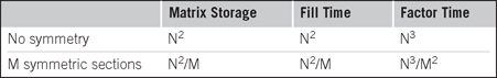
The matrix factor time represents the optimum for a large matrix factored in core. Generally, somewhat longer times will be observed.

• If the structure is added to or modified after the GR command in such a way that cylindrical symmetry is destroyed, the program must be reset to a no-symmetry condition. In most cases, the program is set by the geometry routines for the existing symmetry. The following operations automatically reset the symmetry conditions.
  • Addition of a wire by a GW command destroys all symmetry.
  • Generation of additional structures by a GM command, with NRPT greater than 0, destroys all symmetry.
  • A GM command acting on only part of the structure (having ITS greater than 0) destroys all symmetry.
  • A GX or GR command will destroy all previously established symmetry.
  • If a structure is rotated about either the X- or Y-axis by use of a GM command and a ground plane is specified on the GE command, all symmetry will be destroyed. Rotation about the Z-axis or translation will not affect symmetry. If a ground is not specified, symmetry will be unaffected by any rotation or translation by a GM command, unless NRPT or ITS on the GM command is greater than 0.
• Symmetry will also be destroyed if lumped loads are placed on the structure in an unsymmetric manner. In this case, the program is not automatically set to a no-symmetry condition but must be set by a data command following the GR command. A GW command with NS blank will set the program to a no-symmetry condition without modifying the structure. The command must specify a nonzero radius, however, to avoid reading a GC command.
• Placement of nonradiating networks or sources does not affect symmetry.
• When symmetry is used in the solution, the number of symmetric sections (I2) is limited by array dimensions.
• The GR command produces the same effect on the structure as a GM command if I2 on the GR command is equal to (NRPT + 1) on the GM command and if ROZ on the GM command is equal to 360/(NRPT + 1) degrees. If the GM command is used, however, the program will not be set to take advantage of symmetry.

2.8 Scale Structure Dimensions (GS)

Purpose

To scale all dimensions of a structure by a constant.

Parameters

Integers

The integer fields are not used.

Decimal Numbers

• (F1) — All structure dimensions, including wire radius, are multiplied by F1.

Note

At the end of geometry input, structure dimensions must be in units of meters. Hence, if the dimensions have been input in other units, a GS command must be used to convert to meters.

2.9 Wire Specification (GW, GC)

Purpose

To generate a string of segments to represent a straight wire.

This command defines a string of segments with radius RAD. If RAD is 0 or blank, a second command is read to set parameters to taper the segment lengths and radius from one end of the wire to the other. The format for the second command (GC), which is read only when RAD is 0, is:

Typical Broadcast Application

Parameters of GW Command

Integers

• ITG (I1) — Tag number assigned to all segments of the wire.
• NS (I2) — Number of segments into which the wire will be divided.

Decimal Numbers

• XW1 (F1) — X coordinate of wire end 1.
• YW1 (F2) — Y coordinate of wire end 1.
• ZW1 (F3) — Z coordinate of wire end 1.
• XW2 (F4) — X coordinate of wire end 2.
• YW2 (F5) — Y coordinate of wire end 2.
• ZW2 (F6) — Z coordinate of wire end 2.
• RAD (F7) — Wire radius, or 0 for tapered segment option.

Parameters of Optional GC Command

• RDEL (F1) — Ratio of the length of a segment to the length of the previous segment in the string.
• RAD1 (F2) — Radius of the first segment in the string.
• RAD2 (F3) — Radius of the last segment in the string.

The ratio of the radii of adjacent segments is:

If the total wire length is L, the length of the first segment is

or

Notes

• The tag number is for later use when a segment must be identified, such as when connecting a voltage source or lumped load to the segment. Any number except 0 can be used as a tag. When identifying a segment by its tag, the tag number and the number of the segment in the set of segments having that tag are given. Thus, the tag of a segment does not need to be unique. If no need is anticipated to refer back to any segments on a wire by tag, the tag field may be left blank. This results in a tag of 0, which cannot be referenced as a valid tag.
• If two wires are electrically connected at their ends, then identical coordinates should be used for the connected ends to ensure that the wires are treated as connected for current interpolation. If wires intersect away from their ends, the point of intersection must occur at segment ends within each wire for interpolation to occur. Generally, wires should intersect only at their ends unless the location of segment ends is accurately known.
• The only significance of differentiating end 1 from end 2 of a wire is that the positive reference direction for current will be in the direction from end 1 to end 2 on each segment making up the wire.
• As a rule of thumb, segment lengths should be less than 0.1 wavelength at the desired frequency. Somewhat longer segments may be used on long wires with no abrupt changes, while shorter segments, 0.05 wavelength or less, may be required in modeling critical regions of an antenna.
• If input is in units other than meters, then the units must be scaled to meters through the use of a Scale Structure Dimensions (GS) command (see page 208).

2.10 Reflection in Coordinate Planes (GX)

Purpose

To form structures having planes of symmetry by reflecting part of the structure in the coordinate planes, and to set flags so that symmetry is used in the solution.

Parameters

Integers

• TNI (I1) — Tag number increment.
• XYZ (12) — This integer is divided into three independent digits, in columns 8, 9, and 10, which control reflection in the three orthogonal coordinate planes. A 1 in column 8 causes reflection along the X-axis (reflection in Y, Z plane); a 1 in column 9 causes reflection along the Y-axis; and a 1 in column 10 causes reflection along the Z-axis. A 0 or blank in any of these columns causes the corresponding reflection to be skipped.

Decimal Numbers

The decimal number fields are not used.

Notes

• Any combination of reflections along the X, Y, and Z-axes may be used. For example, 101 for (I2) will cause reflection along axes X and Z, and 111 will cause reflection along axes X, Y, and Z. When combinations of reflections are requested, the reflections are done in reverse alphabetical order. That is, if a structure is generated in a single octant of space and a GX command is then read with I2 equal to 111, the structure is first reflected along the Z-axis; the structure and its image are then reflected along the Y-axis; and, finally, these four structures are reflected along the X-axis to fill all octants. This order determines the position of a segment in the sequence and, hence, the absolute segment numbers.
• The tag increment I1 is used to avoid duplication of tag numbers in the image segments. All valid tags on the original structure are incremented by I1 on the image. When combinations of reflections are employed, the tag increment is doubled after each reflection. Thus, a tag increment greater than or equal to the largest tag on the original structure will ensure that no duplicate tags are generated. For example, if tags from 1 through 100 are used on the original structure with I2 equal to 011 and a tag increment of 100, the first reflection, along the Z-axis, will produce tags from 101 through 200; and the second reflection, along the Y-axis, will produce tags from 201 through 400, as a result of the increment being doubled to 200.
• The GX command should never be used when there are segments located in the plane about which reflection would take place or when segments cross this plane. The image segments would then coincide with or intersect the original segments, and such overlapping segments are not allowed. Segments may end on the image plane, however.
• When a structure having plane symmetry is formed by a GX command, the program will make use of the symmetry to simplify solution for the currents. The following table shows the number of complex numbers in matrix storage and the proportionality factors for matrix fill time and matrix factor time for a structure modeled by N segments.

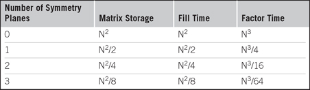
The matrix factor time represents the optimum for a large matrix factored in core. Generally, somewhat longer times will be observed.

• If the structure is added to or modified after the GX command in such a way that symmetry is destroyed, the program must be reset to a no-symmetry condition. In most cases, the program is set by the geometry routines for the existing symmetry. The following operations automatically reset the symmetry condition.
  • Addition of a wire by a GW command destroys all symmetry.
  • Generation of additional structures by a GM command, with NRPT greater than 0, destroys all symmetry.
  • A GM command acting on only part of the structure (having ITS greater than 0) destroys all symmetry.
  • A GX command or GR command will destroy all established symmetry. For example, two GR commands with I2 equal to 011 and 100, respectively, will produce the same structure as a single GX command with I2 equal to 111; however, the first case will set the program to use symmetry about the Y- Z plane only while the second case will make use of symmetry about all three coordinate planes.
  • If a ground plane is specified on the GE command, symmetry about a plane parallel to the X-Y plane will be destroyed. Symmetry about other planes will be used, however.
  • If a structure is rotated about either the X- or Y-axis by use of a GM command and a ground plane is specified on the GE command, all symmetry will be destroyed. Rotation about the Z-axis or translation will not affect symmetry. If a ground is not specified, no rotation or translation will affect symmetry conditions unless NRPT on the GM command is greater than zero.
  • Symmetry will also be destroyed if lumped loads are placed on the structure in an unsymmetric manner. In this case, the program is not automatically set to a no-symmetry condition but must be set by a data command following the GX command. A GW command with NS blank will set the program to a no-symmetry condition without modifying the structure. The command must specify a nonzero radius, however, to avoid reading a GC command.
• Placement of sources or nonradiating networks does not affect symmetry.

2.11 Surface Patch (SP)

Purpose

To input parameters of a single surface patch.

If NS is 1, 2, or 3, a second command is read in the following format:

Parameters

Integers

blank (I1) is not used.

NS (I2) — Selects the patch shape.

0 — (default) arbitrary patch shape

1 — rectangular patch

2 — triangular patch

3 — quadrilateral patch

Decimal Numbers

Arbitrary shape (NS = 0).

• X1 (F1) — X coordinate of patch center.
• Y1 (F2) — Y coordinate of patch center.
• Z1 (F3) — Z coordinate of patch center.
• X2 (F4) — Elevation angle above the X-Y plane of outward normal vector (degrees).
• Y2 (F5) — Azimuth angle from X-axis of outward normal vector (degrees).
• Z2 (F6) — Patch area (square of units used).

Rectangular, triangular, or quadrilateral patch (NS = 1, 2, or 3).

• X1 (F1) — X coordinate of corner 1.
• Y1 (F2) — Y coordinate of corner 1.
• Z1 (F3) — Z coordinate of corner 1.
• X2 (F4) — X coordinate of corner 2.
• Y2 (F5) — Y coordinate of corner 2.
• Z2 (F6) — Z coordinate of corner 2.
• X3 (Fl) — X coordinate of corner 3.
• Y3 (F2) — Y coordinate of corner 3.
• Z3 (F3) — Z coordinate of corner 3.

For the quadrilateral patch only (NS = 3).

• X4 (F4) — X coordinate of corner 4.
• Y4 (F5) — Y coordinate of corner 4.
• Z4 (F6) — Z coordinate of corner 4.

Note

For more detail on the use of surface patches, see NOSC Technical Document 116, Numerical Electromagnetic Code (NEC) — Method of Moments, Part III: User's Guide, available on the Internet at www.ntis.gov.

2.12 Multiple Patch Surface (SM)

Purpose

To cover a rectangular region with surface patches.

A second command with the following format must immediately follow an SM command:

Parameters

Integers

• NX, NY (I1, I2) — The rectangular surface is divided into NX patches from corner 1 to corner 2 and NY patches from corner 2 to corner 3.

Decimal Numbers

• X1, Y1, Z1 (F1, F2, F3) — X,Y,Z coordinates of corner 1.
• X2, Y2, Z2 (F4, F5, F6) — X,Y,Z coordinates of corner 2.
• X3, Y3, Z3 (F1, F2, F3) — X,Y,Z coordinates of corner 3.

Note

For more detail on the use of surface patches see NOSC Technical Document 116, Numerical Electromagnetic Code (NEC) — Method of Moments, Part III: User's Guide, available on the Internet at www.ntis.gov.

3.0 Program Control Commands

The program control commands follow the structure geometry commands. They set electrical parameters for the model, select options for the solution procedure, and request data computation.

There is no fixed order for the program control commands. The desired parameters and options are set first, followed by requests for calculations. Parameters that are not set in the input data are given default values. The one exception to this is the excitation command (EX), which must be set by the user.

Computation of currents may be requested by an XQ command. R P, NE, or NH commands cause calculation of the currents and radiated or near fields on their first occurrence. Subsequent R P, NE, or NH commands cause computation of fields using the previously calculated currents. Any number of near-field and radiation-pattern requests may be grouped together in a data file. An exception to this occurs when multiple frequencies are requested by a single FR command. In this case, only a single NE or NH command and a single RP command will remain in effect for all frequencies.

All parameters retain their values until changed by subsequent data commands. Hence, after parameters have been set and currents or fields computed, selected parameters may be changed and the calculations repeated. For example, if a number of different excitations are required at a single frequency, the file could have the form FR, EX, XQ, EX, XQ, … If a single excitation is required at a number of frequencies, the commands EX, FR, XQ, FR, XQ, … could be used.

The program control commands are explained on the following pages. The format of all program commands has four integers and six floating-point numbers. Not all are used on every command.

3.1 Coupling Calculation (CP)

Purpose

To request the calculation of the maximum coupling between segments identified as TAG1, SEG1 and TAG2, SEG2.

Parameters

TAG1 (I1) & SEG1 (I2) — Specify segment number SEG1 in the set of segments having tag TAG1. If TAG1 is blank or 0, then SEG1 is the absolute segment number.

TAG2 (I3) & SEG2 (I4) — Same as above.

Notes

• Up to five segments may be specified on 2-1/2 CP commands. Coupling is computed between all pairs of these segments. When more than two segments are specified, the CP commands must be grouped together. A new group of CP commands replaces the old group.
• CP does not cause the program to proceed with the calculation but only sets the segment numbers. The specified segments must then be excited (EX command) one at a time in the specified order and the currents computed (XQ, R P, NE, or NH command). The excitation must use the applied-field voltage-source model. When all of the specified segments have been excited in the proper order, the couplings will be computed and printed. After the coupling calculation, the set of CP commands is cancelled.
• When using NEC-2, CP will not return the correct values for segments containing network or transmission line connections. NEC-4 does not suffer this limitation.

3.2 Extended Thin-Wire Kernal (EK)

Purpose

To control use of the extended thin-wire kernel approximation. Without an EK command, the program will use the standard thin-wire kernel.

Typical Broadcast Application

Parameters

Integers

ITMP1 (I1) — Blank or zero to initiate use of the extended thin-wire kernel, — 1 to return to standard thin-wire kernel.

3.3 End of Run (EN)

Purpose

To indicate to the program the end of all execution.

Typical Broadcast Application

EN

Parameters

None.

3.4 Excitation (EX)

Purpose

To specify the excitation for the structure. The excitation can be voltage sources on the structure, an elementary current source, or a plane-wave incident on the structure.

Typical Broadcast Application

Parameters

Integers

(I1) — Determines the type of excitation that is used.

0 — Voltage source (applied-E-field source).

1 — Incident plane wave, linear polarization.

2 — Incident plane wave, right-hand (thumb along the incident k vector) elliptic polarization.

3 — Incident plane wave, left-hand elliptic polarization.

4 — Elementary current source.

5 — Voltage source (current-slope-discontinuity).

Remaining integers depend on excitation type.

a. If I1 is a voltage source of type 0 or 5, then

(I2) — Tag number of the source segment. This tag number, along with the number to be given in (I3), uniquely defines the source segment. Blank or 0 in field (I2) implies that the Source segment will be identified by using the absolute segment number in the next field.

(I3) — Equal to m, specifies the mth segment of the set of segments whose tag numbers are equal to the number set by the previous parameter. If the previous parameter is 0, the number in (I3) must be the absolute segment number of the source.

(I4) — Columns l9 and 20 of this field are used separately. The options for column l9 are:

0 — No action.

1 — Maximum relative admittance matrix asymmetry for source segments and network connections will be calculated and printed.

The options for column 20 are:

0 — No action

1 — The input impedance at voltage sources is always printed directly before the segment currents in the output. By setting this flag, the impedance of a single source segment in a frequency loop will be collected and printed in a table (in a normalized and unnormalized form) after the information at all frequencies has been printed. Normalization to the maximum value is a default, but the normalization value can be specified (refer to F3 under voltage source below). When there is more than one source on the structure, only the impedance of the last source specified will be collected.

b. If I1 is an incident plane wave of type 1, 2, or 3:

(I2) — Number of theta angles desired for the incident plane wave.

(I3) — Number of phi angles desired for the incident plane wave.

(I4) — 0 — no action

1 — maximum relative admittance matrix asymmetry for network connections will be calculated and printed.

c. If I1 is an elementary current source of type 4:

(I2) and (I3) — Blank.

(I4) — Identical to that listed under b.

Floating-Point Options

a. Voltage source (Il = 0 or 5).

(F1) — Real part of the voltage in volts.

(F2) — Imaginary part of the voltage in volts.

(F3) — If a second digit (1) is placed in I4 (see above), this field can be used to specify a normalization constants for the impedance printed in the optional impedance table. Blank in this field produces normalization to the maximum value.

(F4), (F5), and (F6) — blank.

b. Incident plane wave (I1 = 1, 2, or 3). The incident wave is characterized by the direction of incident ^k wave polarization in the plane normal to k.

(F1) — Theta in degrees. Theta is defined in standard spherical coordinates.

(F2) — Phi in degrees. Phi is the standard spherical angle defined in the X-Y plane.

(F3) — Eta in degrees. Eta is the polarization angle defined as the angle between the theta unit vector and the direction of the electric field for linear polarization or the major ellipse axis for elliptical polarization.

(F4) — Theta angle stepping increment in degrees.

(F5) — Phi angle stepping increment in degrees.

(F6) — Ratio of minor axis to major axis for elliptic polarization (major axis field strength — 1 V/m).

c. Elementary current source (I1 = 4). The current source is characterized by its Cartesian coordinate position, orientation, and its magnitude.

(F1) — X position in meters.

(F2) — Y position in meters.

(F3) — Z position in meters.

(F4) — alpha in degrees. alpha is the angle the current source makes with the X-Y plane.

(F5) — beta in degrees. beta is the angle the projection of the current source on the X-Y plane makes with the X-axis.

(F6) — “Current moment” of the source. This parameter is equal to the product current times length in amp meters.

Notes

• In the case of voltage sources, excitation commands can be grouped to specify multiple sources. The maximum number of voltage sources that may be specified is determined by dimension statements in the program.
• The applied-E-field voltage source is located on the segment specified.
• The current-slope-discontinuity source is located at the first end, relative to the reference direction, of the specified segment, at the junction between the specified segment and the previous segment. This Junction must be a simple two-segment junction, and the two segments must be parallel with equal lengths and radii.
• A current-slope-discontinuity voltage source may lie in a symmetry plane. An applied-field voltage source may not lie in a symmetry plane since a segment may not lie in a symmetry plane. An applied-field voltage source may be used on a wire crossing a symmetry plane by exciting the two segments on opposite sides of the symmetry plane, each with half the total voltage, taking account of the reference directions of the two segments.
• An applied-field voltage source specified on a segment that has been impedance-loaded, through the use of an LD command, is connected in series with the loads. An applied-field voltage source specified on the same segment as a network is connected in parallel with the network port. For the specific case of a transmission line, the source is in parallel with both the line and the shunt load. Applied-field voltage sources should be used in these cases since loads and network connections are located on, rather than between, segments.
• Only one incident plane wave or one elementary current source is allowed at a time. Also, plane-wave or current-source excitation is not allowed with voltage sources. If the excitation types are mixed, the program will use the last excitation type encountered.
• When a number of theta and phi angles are specified for an incident plane-wave excitation, the theta angle changes more rapidly than phi.
• The current element source illuminates the structure with the field of an infinitesimal current element at the specified location. The current element source cannot be used over a ground plane.

3.5 Frequency (FR)

Purpose

To specify the frequency(s) in megahertz.

Typical Broadcast Application

Parameters

Integers

IFRQ (I1) — Determines the type of frequency stepping, which is

0 — Linear stepping.

1 — Multiplicative stepping.

NFRQ (12) — Number of frequency steps. If this field is blank, one is assumed.

(I3) and (I4) — Blank.

Floating Point

FMHZ (F1) — Frequency in megahertz.

DELFRQ (F2) — Frequency stepping increment. If the frequency stepping is linear, this quantity is added to the frequency each time. If the stepping is multiplicative, this is the multiplication factor.

(F3) through (F6) — Blank.

Notes

• If a frequency command does not appear in the data file, a single frequency of 299.8 MHz is assumed. Since the wavelength at 299.8 MHz is 1 meter, the geometry is in units of wavelengths for this case.
• Frequency commands may not be grouped together. If they are, only the information on the last command in the group will be used.
• After an FR command with NFRQ greater than 1, an NE or NH command will not initiate execution but an RP or XQ command will. In this case, only one NE or NH command and one RP command will be effective for the multiple frequencies.
• After a frequency loop for NFRQ greater than 1 has been completed, it will not be repeated for a second execution request. The FR command must be repeated in that case.

3.6 Additional Ground Parameters (GD)

Purpose

To specify the ground parameters of a second medium, which is not in the immediate vicinity of the antenna. This command may only be used if a GN command has also been used. It does not affect the field of surface patches.

Typical Broadcast Application

Parameters

Integers

All integer fields are blank.

Floating Point

EPSR2 (F1) — Relative dielectric constant of the second medium.

SIG2 (F2) — Conductivity in mhos/mecer of the second medium.

CLT (F3) — Distance in meters from the origin of the coordinate system to the join between medium 1 and 2. This distance is either the radius of the circle where the two media join, or the distance out the plus X-axis to where the two media join in a line parallel to the Y-axis. Specification of the circular or linear option is on the RP command.

CHT (F4) — Distance in meters (positive or 0) by which the surface of medium 2 is below medium 1.

Notes

• The GD command can only be used in a data file where the GN command has been used since the GN command is the only way to specify the ground parameters in the vicinity of the antenna (see GN command write-up). However, a number of GD commands may be used in the same data file with only one GN command.
• GD commands may not be grouped together. If they are, only the information on the last command of the group is retained.
• When a second medium in specified, a flag must also be set on the radiation pattern (RP) data command in order to calculate the patterns including the effect of the second medium. Refer to the radiation-pattern command write-up for details.
• Use of the GD command does not require recalculation of the matrix or currents.
• The parameters for the second medium are used only in the calculation of the far-fields. It is possible then to set the radius of the boundary between the two media equal to 0 and thus have the far-fields calculated by using only the parameters of medium 2. The currents for this case will still have been calculated by using the parameters of medium 1.
• When a model includes surface patches, the fields due to the patches will be calculated by using only the primary ground parameters. Hence, a second ground medium should not be used with patches.

3.7 Ground Parameters (GN)

Purpose

To specify the relative dielectric constant and conductivity of ground in the vicinity of the antenna. In addition, a second set of ground parameters for a second medium can be specified, or a radial wire ground screen can be modeled using a reflection coefficient approximation.

Typical Broadcast Application

Parameters

Integers

IPERF (I1) — Ground-type flag. The options are:

— 1 — Nullifies ground parameters previously used and sets free-space condition. The remainder of the command is left blank in this case.

0 — Finite ground, reflection coefficient approximation.

1 — Perfectly conducting ground.

2 — Finite ground, Sommerfeld/Norton method.

NRADL (I2) — Number of radial wires in the ground screen approximation; blank or 0 implies no ground screen.

(I3) and (I4) — Blank.

Floating Point

EPSE (F1) — Relative dielectric constant for ground in the vicinity of the antenna. Leave blank in case of a perfect ground.

SIG (F2) — Conductivity in mhos/meter of the ground in the vicinity of the antenna. Leave blank in the case of a perfect ground. If SIG is input as a negative number, the complex dielectric constant is set to EPSR — j |SIG|.

Options for Remaining Floating Point Fields (F3–F6)

a. For the case of an infinite ground plane, F3 through F6 are blank.

b. Radial wire ground screen approximation (NRADL ≠ 0). The ground screen is always centered at the origin, that is, (0, 0, 0) and lies in the X-Y plane.

P1 (F3) — The radius of the screen in meters.

P2 (F4) — Radius of the wires used in the screen in meters.

P3 (F5) — blank.

P4 (F6) — blank.

c. Second medium parameters (NRADL = 0) for medium outside the region of the first medium (cliff problem). These parameters alter the far-field patterns but do not affect the antenna impedance or current distribution.

P1 (F3) — Relative dielectric constant of medium 2.

P2 (F4) — Conductivity of medium 2 in mhos/meter.

P3 (F5) — Distance in meters from the origin of the coordinate system to the boundry between medium 1 and 2. This distance is either the radius of the circle where the two media join, or the distance out the positive X-axis to where the two media join in a line parallel to the Y-axis. Specification of the circular or linear option is on the RP command.

P4 (F6) — Distance in meters (positive or 0) by which the surface of medium 2 is below medium 1.

Notes

• When the Sommerfeld/Norton method is used, many NEC-2 codes require an input-data file that is generated by the program SOMNEC for the specific ground parameters and frequency. SOMNEC is integrated into bnec.exe, however, and is run transparently when needed. The file generated by SOMNEC depends only on the complex dielectric constant. NEC-2 compares the complex dielectric constant from the file with that determined by the GN command parameters and frequency. If the relative difference exceeds 10⁻³, an error message is printed. Once the SOMNEC data file has been read for the first use of the Sommerfeld/Norton method, the data is retained until the end of the run. Subsequent data, including new data sets following NX commands, may use the SOMNEC data file if the ground parameters and frequency remain unchanged. Other ground options may be intermixed with the Sommerfeld/Norton option.
• The parameters of the second medium can also be specified on another data command whose mnemonic is GD. With the GD command, the parameters of the second medium can be varied and only the radiated fields need to be recalculated. Furthermore, if a radial wire ground screen has been specified on the GN command, the GD command is the only way to include a second medium. See the write-up of the GD command for details.
• GN commands may not be grouped together. If they are, only the information on the last command will be retained.
• Use of a GN command after any form of execute dictates structure matrix regeneration.
• Only the parameters of the first medium are used when the antenna currents are calculated; the parameters associated with the second medium are not used until the calculation of the far-fields. It is possible then to calculate the currents over one set of ground parameters (medium 1), but to calculate the far-fields over another set (medium 2) by setting the distance to the start of medium 2 to 0. Medium 1 can even be a perfectly conducting ground specified by IPERF = 1.
• When a radial-wire ground screen or a second medium is specified, it is necessary to indicate their presence by the first parameter on the RP command in order to generate the proper radiation patterns.
• When a ground plane is specified, this fact should also be indicated on the GE command. Refer to the GE command for details.
• When a model includes surface patches, the fields due to the patches will be calculated by using only the primary ground parameters. Hence, a second ground medium should not be used with patches. The radial-wire ground screen approximation also is not implemented for patches.

3.8 Interaction Approximation Range (KH)

Purpose

To set the minimum separation distance for use of a time-saving approximation in filling the interaction matrix.

Parameters

Integers

None.

Decimal Numbers

RKH (F1) — The approximation is used for interactions over distances greater than RKH wavelengths.

Notes

• If two segments or a segment and a patch are separated by more than RKH wavelengths, the interaction field is computed from an impulse approximation to the segment current. The field of a current element located at the segment center is used. No approximation is used for the field due to the surface current on a patch since the time for the standard calculation is very short.
• The KH command can be placed anywhere in the data file following the geometry commands (with FR, EX, LD, etc.) and affects all calculations requested following its occurrence. The value of RKH may be changed within a data set by use of a new KH command.

3.9 Loading (LD)

Purpose

To specify the impedance loading on one segment or a number of segments. Series and parallel RLC circuits can be generated. In addition, a finite conductivity can be specified for segments.

Typical Broadcast Application

Parameters

Integers

LDTYP (I1) — Determines the type of loading used. The options are:

— 1 — short all loads (used to nullify previous loads). The remainder of the command is left blank.

0 — series RLC, input ohms, henries, farads.

1 — parallel RLC, input ohms, henries, farads.

2 — series RLC, input ohms/meter, henries/meter, farads/meter.

3 — parallel RLC, input ohms/meter, henries/meter, farads/meter.

4 — impedance, input resistance and reactance in ohms.

5 — wire conductivity, mhos/meter.

LDTAG (I2) — Tag number; identifies the wire section(s) to be loaded by its (their) tag numbers. The next two parameters can be used to further specify certain segment(s) on the wire section(s). Blank or 0 here implies that absolute segment numbers are being used in the next two parameters to identify segments. If the next two parameters are blank or 0, all segments with tag LDTAG are loaded.

LDTAGF (I3) — Equal to m specifies the mth segment of the set of segments whose tag numbers equal the tag number specified in the previous parameter. If the previous parameter (LDTAG) is 0, LDTAGF then specifies an absolute segment number. If both LDTAG and LDTAGF are 0, all segments will be loaded.

LDTAGT (I4) — Equal to n specifies the nth segment of the set of segments whose tag numbers equal the tag number specified in the parameter LDTAG. This parameter must be greater than or equal to the previous parameter. The loading specified is applied to each of the mth through nth segments of the set of segments having tags equal to LDTAG. Again, if LDTAG is zero, these parameters refer to absolute segment numbers. If LDTAGT is left blank, it is set equal to the previous parameter (LDTAGF).

Floating Point — Input for the Various Load Types

a. Series RLC (LDTYP = 0)

ZLR (Fl) — Resistance in ohms; if none, 0 or leave blank.

ZLI (F2) — Inductance in henries; if none, 0 or leave blank.

ZLC (F3) — Capacitance in farads; if none, 0 or leave blank.

b. Parallel RLC (LDTYP = 1).

Floating point inputs same as in item a.

c. Series RLC (LDTYP = 2) input, parameters per unit length.

ZLR — Resistance in ohms/meter; if none, 0 or leave blank.

ZLI — Inductance in henries/meter; if none, 0 or leave blank.

ZLC — Capacitance in farads/meter; if none, 0 or leave blank.

d. Parallel RLC (LDTYP = 3), input parameters per unit length, floating point input same as in item c.

e. Impedance (LDTYP = 4).

ZLR — Resistance in ohms.

ZLI — Reactance in ohms.

f. Wire conductivity (LDTYP = 5).

ZLR — Conductivity in mhos/meter.

Notes

• Loading commands can be input in groups to achieve a desired structure loading. The maximum number of loading commands in a group is determined by dimensions in the program.
• If a segment is loaded more than once by a group of loading commands, the loads are assumed to be in series (impedances added), and a comment is printed in the output alerting the user to this fact.
• When resistance and reactance are input (LDTYP = 4), the impedance does not automatically scale with frequency.
• Loading commands used after any form of execute, require the regeneration of the structure matrix.
• Since loading modifies the interaction matrix, it will affect the conditions of plane or cylindrical symmetry of a structure. If a structure is geometrically symmetric and each symmetric section is to receive identical loading, then symmetry may be used in the solution. The program is set to use symmetry during geometry input by inputting the data for one symmetric section and completing the structure with a GR or GX command. If symmetry is used, the loading on only the first symmetric section is input on LD commands. The same loading will be assumed on the other sections. Loading should not be specified for segments beyond the first section when symmetry is used. If the sections are not identically loaded, then during geometry input the program must be set to a no-symmetry condition to permit independent loading of corresponding segments in different sections.

3.10 Near Fields (NE, NH)

Purpose

To request calculation of near electric fields in the vicinity of the antenna (NE) or to request near magnetic fields (NH). Use NE or NH as appropriate.

Parameters

Integers

NEAR (I1) — Coordinate system type. The options are:

0 — Rectangular coordinates will be used.

1 — Spherical coordinates will be used.

Remaining integers depend on coordinate type.

a. Rectangular coordinates (NEAR = 0).

NRX, NRY, NRX (I2, I3, I4) — Number of points desired in the X, Y, and Z directions, respectively. X changes the most rapidly, then Y, and then Z. The value 1 is assumed for any field left blank.

b. Spherical coordinates (NEAR = 1).

(I2, I3, I4) — Number of points desired in the r, phi, and theta directions, respectively. r changes the most rapidly, then phi, and then theta. The value 1 is assumed for any field left blank.

Floating Point Fields

Their specification depends on the coordinate system chosen.

a. Rectangular coordinates (NEAR = 0).

XNR, YNR, ZNR (F1, F2, F3) — The (X, Y, Z) coordinate position (F1, F2, F3), respectively, in meters of the first field point.

DXNR, DYNR, DZNR (F4, F5, F6) — Coordinate stepping increment in meters for the X, Y, and Z coordinates (F4, F5, F6), respectively. In stepping, X changes most rapidly, then Y, and then Z.

b. Spherical coordinates (NEAR = 1).

(F1, F2, F3) — The (r, phi, theta) coordinate position (Fl, F2, F3), respectively, of the first field point. r is in meters, and phi and theta are in degrees.

(F4, F5, F6) — Coordinate stepping increments for r, phi, and theta (F4, F5, F6), respectively. The stepping increment for r is in meters and for phi and theta, it is in degrees.

Notes

• When only one frequency is being used, near-field commands may be grouped together in order to calculate fields at points with various coordinate increments. For this case, each command encountered produces an immediate execution of the near-field routine and the results are printed. When automatic frequency stepping is being used (i.e., when the number of frequency steps [NFRQ] on the FR command is greater than one), only one NE or NH command can be used for program control inside the frequency loop. Furthermore, the NE or NH command does not cause an execution in this case. Execution will begin only after a subsequent radiation-pattern command (RP) or execution command (XQ) is encountered (see write-ups on both of these commands).
• The time required to calculate the field at one point is equivalent to filling one row of the matrix. Thus, if there are N segments in the structure, the time required to calculate fields at N points is equivalent to the time required to fill an N x N interaction matrix.
• The near electric field is computed by whichever form of the field equations selected for filling the matrix, either the thin-wire approximation or extended thin-wire approximation. At large distances from the structure, the segment currents are treated as infinitesimal current elements.
• If the field calculation point falls within a wire segment, the point is displaced by the radius of that segment in a direction normal to the plane containing each source segment and the vector from that source segment to the observation segment. When the specified field-calculation point is at the center of a segment, this convention is the same as is used in filling the interaction matrix. If the field point is on a segment axis, that segment produces no contribution to the H-field or the radial component of the E-field. If these components are of interest, the field point should be on or outside of the segment surface.

3.11 Networks (NT)

Purpose

To generate a two-port nonradiating, network connected between any two segments in the structure. The characteristics of the network are specified by its short-circuit admittance matrix elements. For the special case of a transmission line, a separate command is provided for convenience, although the mathematical method is the same as for networks. Refer to the TL command.

Typical Broadcast Application

Parameters

Integers

TAG1 (I1) — Tag number of the segment to which port 1 of the network is connected. This tag number along with the number to be given in (I2), which identifies the position of the segment in a set of equal tag numbers, uniquely defines the segment for port 1. Blank or 0 here implies that the segment will be identified, using the absolute segment number in the next location (12).

SEG1 (I2) — Equal to m, specifies the mth segment of the set of segments whose tag numbers are equal to the number set by the previous parameter. If the previous parameter is 0, the number in (12) is the absolute segment number corresponding to end 1 of the network. A minus one in this field will nullify all previous network and transmission line connections. The rest of the command is left blank in this case.

TAG2 (I3) — Used in exactly the same way as (I1) and (I2) in order to specify the segment corresponding to port 2 of the network connection.

SEG2 (I4) — As above.

Floating Point

The six floating-point fields are used to specify the real and imaginary parts of three short-circuit admittance matrix elements (1, 1), (1, 2), and (2, 2), respectively. The admittance matrix is symmetric so it is unnecessary to specify element (2, 1).

• Y11R (F1) — Real part of element (1, 1) in mhos.
• Y11I (F2) — Imaginary part of element (1, 1) in mhos.
• Y12R (F3) — Real part of element (1, 2) in mhos.
• Y12I (F4) — Imaginary part of element (1, 2) in mhos.
• Y22R (F5) — Real part of element (2, 2) in mhos.
• Y22I (F6) — Imaginary part of element (2, 2) in mhos.

Notes

• Network commands may be used in groups to specify several networks on a structure. All network commands for a network configuration must occur together with no other commands (except TL commands) separating them. When the first NT command is read following a command other than an NT or TL command, all previous network and transmission line data are destroyed. Hence, if a set of network data is to be modified, all network data must be input again in the modified form. Dimensions in the program limit the number of networks that may be specified. In the present NEC-2 deck, the number of two-port networks (including transmission lines) is limited to thirty, and the number of different segments having network ports connected to them is limited to thirty.
• One or more network ports can be connected to any given segment. Multiple network ports connected to one segment are connected in parallel.
• If a network is connected to a segment that has been impedance loaded (i.e., through the use of the LD command), the load acts in series with the network port.
• A voltage source specified on the same segment as a network port is connected in parallel with the network port.
• Segments can be impedance-loaded by using network commands. Consider a network connected from the segment to be loaded to some other arbitrary segment, as shown in Figure 5.2(c) on page 55. The admittance matrix elements are Y₁₁ = 1/Z_l, Y₁₂ = 0, and Y₂₂ = infinity (computationally a very large number such as 10¹⁰). The advantage of using this technique for loading Ls is that the load can be changed without causing a recalculation of the structure matrix as required when LD commands are used. Furthermore, in some cases a higher degree of structure matrix symmetry can be preserved because the matrix elements are not directly modified by networks, as they are when using the LD commands. (Consider, for instance, a loop with one load where the loop is rotationally symmetric until the load is placed on it.) The disadvantage of the NT command form of loading is that the user must calculate the load admittance, and this value does not automatically scale with frequency. Obviously, in the above schematic, replacing the short with an impedance would load two segments. At a segment at which a voltage source is specified, the effect of loading by the LD and NT commands differs, however, since the network is in parallel with the voltage source while the load specified by an LD command is in series with the source.
• Use of network commands (NT) after any form of execute requires the recalculation of the current only.
• NT and TL commands do not affect structure symmetry.

3.12 Next Structure (NX)

Purpose

To signal the end of data for one structure and the beginning of data for the next.

Parameters

NX appears in the first two columns, and the rest of the command is blank.

Note

The command that directly follows the NX command must be a comment command; CM or CE.

3.13 Print Control for Charge on Wires (PQ)

Purpose

To control the printing of charge densities on wire segments.

Parameters

Integers

IPTFLQ (I1) — Print control flag

— 1 — Suppress printing of charge densities. This is the default condition.

0 (or blank) — Print charge densities on segments specified by the following parameters. If the following parameters are blank, charge densities are printed for all segments.

IPTAQ (I2) — Tag number of the segments for which charge densities will be printed.

IPTAQF (I3) — Equal to m specifies the mth segment of the set of segments having tag numbers of IPTAQ. If IPTAQ is 0 or blank, then IPTAQF refers to an absolute segment number. If IPTAQF is left blank, then charge density is printed for all segments.

IPTAQT (I4) — Equal to n, specifies the nth segment of the set of segments having tag numbers of IPTAQ. Charge densities are printed for segments having tag number IPTAQ starting at the mth segment in the set and ending at the nth segment. If IPTAQ is zero or blank, then IPTAQF and IPTAQT refer to absolute segment numbers. If IPTAQT refer to absolute segment numbers. If IPTAQT is left blank, it is set equal to IPTAQF

Floating Point

Floating-point fields are not used.

3.14 Data Storage for Plotting (PL)

Purpose

To write selected output data into a predesignated file for later plotting.

Parameters

Integers

IPLP1 (I1) — Data type to be written into auxiliary file:

0 — No action.

1 — Wire currents.

2 — Near fields.

3 — Far-field patterns.

4 — Impedance, SWR.

5 — Admittance, SWR.

Remaining integers depend on data type(IPLP1):

a. Wire Currents (IPLP1 = 1).

IPLP2 (format) = 0 — No action

   = 1 — Use real and imaginary format

   = 2 — Use magnitude and phase format

IPLP3 (patch I components) = 0 — No action

= 1 — Ix

= 2 — Iy

= 3 — Iz

= 4 — Ix, Iy, Iz

(all measured in magnitude and phase)

b. Near-Fields (IPLP1 = 2)

IPLP2 (format) = 0 — No action.

= 1 — Use real and imaginary format.

= 2 — Use magnitude and phase format.

IPLP3 (components) = 0 — No action.

= 1 — X component.

= 2 — Y component.

= 3 — Z component.

= 4 — X, Y, Z component.

= 5 — Total field (magnitude only)

IPLP4 (coordinates) = 1 — X coordinate

= 2 — Y coordinate

= 3 — Z coordinate

c. Far-Field Patterns (IPLP1 = 3).

IPLP2 (Angle to be stored) = 1 — Theta or Z

= 2 — Phi

= 3 — Rho

IPLP3 (E-field component) = 0 — No action

= 1 — E(Theta)

= 2 — E(Phi)

= 3 — E(Rho)

(all in magnitude and phase)

IPLP4 (Power pattern) = 0 — No action

= 1 — Vertical gain in dB.

= 2 — Horizontal gain in dB.

= 3 — Total gain in dB.

= 4 — Vertical, horizontal, and total gain in dB.

Notes

1. The PL command may be used anywhere between the GE and XQ commands.
2. A PL command with IPLP1 = 0 will suspend any previous PL specs.
3. All the data requested is written out to a prenamed file.

3.15 Print Control (PT)

Purpose

To control the printing of currents on wire segments. Current printing can be suppressed or limited to a few segments, or special formats for receiving patterns can be requested.

Parameters

Integers

IPTFLG (I1) — Print control flag; specifies the type of format used in printing segment currents. The options are:

— 2 — All currents printed. This it a default value for the program if the command is omitted.

— 1 — Suppress printing of all wire segment currents.

0 — Current printing will be limited to the segments specified by the next three parameters.

1 — Currents are printed by using a format designed for a receiving pattern. Only currents for the segments specified by the next three parameters are printed.

2 — Same as for 1 above; in addition, however, the current for one segment will be normalized to its maximum, ant the normalized values along with the relative strength in dB will be printed in a table. If the currents for more than one segment are being printed, only currents from the last segment in the group appear in the normalized table.

3 — Only normalized currents from one segment are printed for the receiving pattern case.

IPTAG (I2) — Tag number of the segments for which currents will be printed.

IPTAGF (I3) — Equal to m, specifies the mth segment of the set of segments having the tag numbers of IPTAG, at which printing of currents starts. If IPTAG is 0 or blank, then IPTAGF refers to an absolute segment number. If IPTAGF is blank, the current is printed for all segments.

IPTAGT (I4) — Equal to n specifies the nth segment of the set of segments having tag numbers of IPTAG. Currents are printed for segments having tag number IPTAG starting at the mth segment in the set and ending at the nth segment. If IPTAG is 0 or blank, then IPTAGF and IPTAGT refer to absolute segment numbers. In IPTAGT is left blank, it is set to IPTAGF.

Note

For suppressing current print — PT, −1,1,1,1

3.16 Radiation Pattern (RP)

Purpose

To specify radiation pattern sampling parameters and to cause program execution. Options for a field computation include a radial-wire ground screen, a cliff, or surface-wave fields.

Typical Broadcast Application

Parameters

Integers

MOD (I1) — This integer selects the mode of calculation for the radiated field. Some values of (I1) will affect the meaning of the remaining parameters in the command. Options available for I1 are:

0 — Normal mode. Space-wave fields are computed. An infinite ground plane is included if it has been specified previously on a GN command; otherwise, antenna is in free space.

1 — Surface wave propagating along ground is added to the normal space wave. This option changes the meaning of some of the other parameters on the RP cart as explained below, and the results appear in a special output format. Ground parameters must have been input on a GN command.

The following options cause calculation of only the space wave but with special ground conditions. Ground conditions include a two-medium ground (cliff) where the media join in a circle or a line, and a radial-wire ground screen. Ground parameters and dimensions must be input on a GN or GD command before the RP command is read. The RP command only selects the option for inclusion in the field calculation. (Refer to the GN and GD commands for further explanation.)

2 — Linear cliff with antenna above upper level. Lower medium parameters are as specified for the second medium on the GN cart or on the GD command.

3 — Circular cliff centered at origin of coordinate system: with antenna above upper level. Lower medium parameters are as specified for the second medium on the GN command or on the GD command.

4 — Radial-wire ground screen centered at origin.

5 — Both radial-wire ground screen and linear cliff.

6 — Both radial-wire ground screen and circular cliff.

The field point is specified in spherical coordinates (r, sigma, theta) except when the surface wave is computed. For computing the surface-wave field (MOD (Il) = l), cylindrical coordinates (phi, theta, z) are used to accurately define points near the ground plane at large radial distances. The RP command allows automatic stepping of the field point to compute the field over a region about the antenna at uniformly spaced points. The integers I2 and I3 and floating-point numbers Fl, F2, F3, and F4 control the field-point stepping.

NTH (I2) — Number of values of theta (e) at which the field is to be computed (number of values of z for I1 = l).

NPH (I3) — Number of values of phi (f) at which field is to be computed. The total number of field points requested by the command is NTH x NPH. If I2 or I3 is left blank, a value of 1 will be assumed.

XNDA (14) — This optional integer consists of four independent digits, each having a different function. The mnemonic XNDA is not a variable name in the program. Rather, each letter represents a mnemonic for the corresponding digit in I4. If I1 = 1, then I4 has no effect and should be left blank.

X (the first digit) — controls output format.

X = 0 — major axis, minor axis and total gain printed.

X = l — vertical, horizontal ant total gain printed.

N (second digit) — Causes normalized gain for the specified field points to be printed after the standard gain output. The number of field points for which the normalized gain can be printed is limited by an array dimension in the program. In the demonstration program, the limit is 600 points. If the number of field points exceeds this limit, the remaining points will be omitted from the normalized gain. The gain may be normalized to its maximum or to a value input in field F6. The type of gain that is normalized is determined by the value of N as follows:

N = 0 — No normalized gain.

    = 1 — Major axis gain normalized.

    = 2 — Minor axis gain normalized.

    = 3 — Vertical axis gain normalized.

    = 4 — Horizontal axis gain normalized.

    = 5 — Total gain normalized.

D (the third digit) — Selects either power gain or directive gain for both standard printing and normalization. If the structure excitation is an incident plane wave, the quantities printed under the heading “gain” will actually be the scattering cross section (a/λ²) and will not be affected by the value of D. The column heading for the output will still read “power” or “directive gain,” however.

D = 0 — Power gain.

    = 1 — Directive gain.

A — (the fourth digit) — Requests calculation of average power gain over the region covered by field points.

A = 0 — No averaging.

    = 1 — Average gain computed.

    = 2 — Average gain computed; printing of gain at the field points used for averaging is suppressed. If NTH or NPH is equal to one, average gain will not be computed for any value of A since the area of the region covered by field points vanishes.

Floating Point Numbers

THETS (F1) — Initial theta angle in degrees (initial z coordinate in meters if I1 = 1).

PHIS (F2) — Initial phi angle in degrees.

DTH (F3) — Increment for theta in degrees (increment for z in meters if I1 = 1).

DPH (F4) — Increment for phi in degrees.

RFLD (F5) — Radial distance (R) of field point from the origin in meters. RFLD is optional. If it is blank, the radiated electric field will have the factor exp(-jkR)/R omitted. If a value of R is specified, it should represent a point in the far-field region since near components of the field cannot be obtained with an RP command. (If I1 = 1, then RFLD represents the cylindrical coordinate phi in meters and is not optional. It must be greater than about one wavelength.)

GNOR (F6) — Determines the gain normalization factor if normalization has been requested in the I4 field. If GNOR is blank or 0, the gain will be normalized to its maximum value. If GNOR is not 0, the gain will be normalized to the value of GNOR.

Notes

• The RP command will initiate program execution, causing the interaction matrix to be computed and factored, and the structure currents to be computed if these operations have not already been performed. Hence, all required input parameters must be set before the RP command is read.
• At a single frequency, any number of RP commands may occur in sequence so that different field-point spacings may be used over different regions of space. If automatic frequency stepping is being used (i.e., NFRQ on the FR command is greater than 1), only one RP command will act as data inside the loop. Subsequent commands will calculate patterns at the final frequency.
• When both NTH and NPH are greater than 1, the angle theta (or Z) will be stepped faster than phi. When a ground plane has been specified, field points should not be requested below the ground (theta greater than 90 degrees or Z less than 0.)

3.17 Transmission Line (TL)

Purpose

To generate a transmission line between any two points on the structure. Characteristic impedance, length, and shunt admittance are the defining parameters.

Typical Broadcast Application

Parameters

Integers

I1 and I2 — Tag and segment number to which end 1 is connected (see NT command).

I3 and I4 — Tag and segment number to which end 2 is connected (see NT command).

Floating Point

(F1) — The characteristic impedance of the transmission line in ohms. A negative sign in front of the characteristic impedance will act as a flag for generating the transmission line with a 180 degree phase reversal (crossed line) if this is desired.

(F2) — The length of transmission line in meters. If this field is left blank, the program will use the straight-line distance between the specified connection points.

The remaining four floating-point fields are used to specify the real and imaginary parts of the shunt admittances at end one and two, respectively.

(F3) — Real part of the shunt admittance in mhos at end 1.

(F4) — Imaginary part of the shunt admittance in mhos at end 1.

(F5) — Real part of the shunt admittance in mhos at end 2.

(F6) — Imaginary part of the shunt admittance in mhos at end 2.

Notes

• The rules for transmission line lines are the same as for network lines. All transmission line commands for a particular transmission line configuration must occur together with no other commands (except NT commands) separating than. When the first TL or NT command is read following a command other than a TL or NT command, all previous network or transmission line data are destroyed. Hence, if a set of TL commands is to be modified, all transmission line and network data must be input again in the modified form. Dimensions in the program limit the number of commands in a group that may be specified. In the NEC-2 demonstration deck, the number of two-port networks (specified by NT commands and TL commands) is limited to thirty, and the number of segments having network ports connected to them is limited to thirty.
• One or more networks (including transmission lines) may be connected to any given segment. Multiple network ports connected to one segment are connected in parallel.
• If a transmission line is connected to a segment that has been impedance-loaded (i.e., through the use of an LD command), the load acts in series with the line.
• Use of transmission line commands (TL) after any form of execute requires the recalculation of the current only and does not require recalculation of the matrix.
• NT and TL commands do not affect symmetry.

3.18 Write NGF File (WG)

Purpose

To write a NGF file for a structure.

Typical broadcast Application

WG

Parameters

None.

3.19 Execute (XQ)

Purpose

To cause program execution at points in the data stream where execution is not automatic. Options on the command also allow for automatic generation of radiation patterns in either of two vertical cuts.

Typical Broadcast Application

XQ

Parameters

Integers

(I1) Options controlled by (I1) are:

0 — No patterns requested (normal case).

1 — Generates a pattern cut in the X-Z plane, i.e., phi = 0 degrees and theta varies from 0 degrees to 90 degrees in 1-degree steps.

2 — Generates a pattern cut in the Y-Z plane, i.e., phi = 90 degrees theta varies from 0 degrees to 90 degrees in 1-degree steps.

3 — Generates both of the cuts described for the values 1 and 2.

The remainder of the command is blank.

Notes

• For the case of a single frequency step, four commands will automatically produce program execution (i.e., the program stops reading data and proceeds with the calculations requested to that point); the four commands are the execute command (XQ), the near-field commands (NE, NH), and the radiation-pattern command (RP). Thus, the only time the XQ command is mandatory, for the case of one frequency, is when only currents and impedances for the structure are desired. On the other hand, for the case of automatic frequency stepping, only the XQ command and the RP command cause execution. Thus, if only near-fields or currents are desired, the XQ command is mandatory to cause execution. Furthermore, the XQ command can always be used as a divider in the data after a command that produces an execute. For instance, if the user wished to put a blank XQ command after an RP command to more easily divide the data into execution groups, the XQ command would act as a do-nothing command.
• The radiation-pattern generation option of the XQ command must not be used when a radial-wire ground screen or a second medium has been specified. For these cases, the RP command is used where the presence of the additional ground parameters is indicated.