
8.1 Objective
One of the objects of a NEC-2 analysis is to calculate a close approximation of an array's driving point impedances when the array elements are in the active condition. In this instance, the active condition is defined as the condition that exists when the elements are driven by the currents and phases that yield the desired pattern. In association with that objective, it is generally believed that if the array elements are modeled such that their calculated self-impedances match the measured self-impedances of the elements of the physical array under passive conditions (i.e., with no drive currents applied) then, because the components involved comprise a linear system, those models will prevail under active conditions. Consequently, towers so modeled may be used in the array calculations to obtain a better estimate of the active drive point impedances.
A common practice, then, is to attempt to adjust the parameters of the tower models such that the calculated self-impedances match, or nearly match, the measured self-impedance of the physical towers. This process is referred to as “modeling by measurement” and is the subject of this chapter.
Unfortunately, the impedance as calculated by NEC-2 is probably the least acceptable parameter being determined by a NEC-2 analysis. Although the calculated impedance is quite adequate to use in designing the antenna-matching networks, in many cases it falls short of the accuracy needed to predict the antenna monitor readings from the calculated base drive currents. This is due not only to physical modeling errors caused by simplifying the model (round wire approximations, unequal radii at segment junctions, small loops, etc.) but also to inherent shortcomings within the NEC-2 computer code, such as the compromised means to mathematically represent the source voltage and the simplified representations of current flow in the conductors.
The data plotted in Figure 8-1 is similar to that in a paper titled “A Study of AM Tower Base Impedance” given by J. B. Hatfield at the 42nd Annual IEEE Broadcast Symposium, September 17, 1992. At the time of this writing, a copy of that paper and other useful information is available at http://www.hatdaw.com/downloads.html. The graph is presented here to show the manner in which the self-impedance of an isolated tower varies with height and to serve as a reference point when considering the graphs in the following sections.
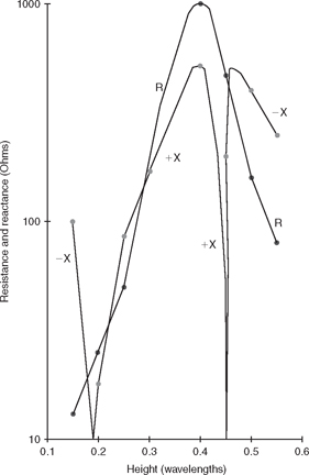
FIGURE 8-1![]()
Typical measured self-impedance of an isolated tower.
8.2 Adjusting the Model
Although it might not be essential to have an exact match between the calculated and measured self-impedance, there are occasions where some analysts may find it desirable to make parameter adjustments during calculations so as to force an acceptable comparison with measured data. The key word here is “force” because in many instances analysts have used artificial means (such as varying tower height) to create a match in the belief that it was beneficial. In reality, the only change may be to eliminate a “wrong answer” in favor of a “more satisfactory wrong answer.” It is important, therefore, that all adjustments be logical and that they be made with discretion.
Reasonable adjustments normally concern only discretionary parameters or parameters that must be estimated because they cannot be measured conveniently. These may include the number and length of wire segments used in the NEC-2 calculations, the assumed equivalent radius of a triangular tower, the assumed effective radius and shunt reactance of the base insulator, the stray capacity and inductance associated with the measuring apparatus, parasitic effects, losses, and so forth. It is not wise to adjust such fundamental parameters as tower height to force the calculated data to agree with measured data because such adjustments might change the current distribution on the towers and distort the conclusions that may be drawn from the analysis. Moreover, the adjustment of fundamental parameters does not appear to make a significant contribution to the final results of an array analysis, so the value of such adjustments appears questionable.
Finally, realistic adjustments are divided into two categories—those associated with the modeled tower and those associated with the measuring apparatus. The latter include such things as test lead inductance and clip lead resistance. Adjustments associated with the tower will, of course, be included in the modeled array. Adjustments associated with the measuring apparatus must be removed when the model tower is incorporated into the array analysis.
The sections in this chapter demonstrate how several parameters might affect the self-impedance of a radiator. It is important to realize that the data displayed by the charts show general trends of a single isolated tower and should not be interpreted as being specific values applicable to any particular configuration or array situation.
8.2.1 Number of Segments
Figures 8-2(a), (b), and (c) show the self-impedance of an isolated tower of fixed height as calculated by NEC-2 using various number of segments ranging from 20 to 100. For all three figures, the tower height is fixed at approximately a quarter wavelength; G = 50 meters at a wavelength of 199.87 meters (1500 KHz). The figures show the results for towers of three different radii.
Figure 8-2(a) illustrates the impedance versus the number of segments for a typical broadcast tower having an equivalent radius of 0.29 meter. This corresponds to a triangular tower with a 24-inch face. It is quite evident from this figure that increasing the number of segments beyond 20 has little effect on the calculated impedance.
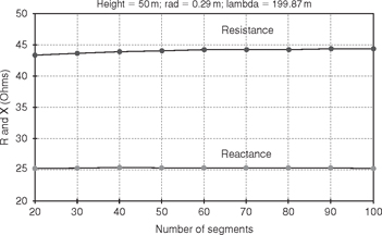
FIGURE 8-2(a)![]()
Segmentation on a typical tower.
Another interesting revelation from this figure is that the guidelines for tower modeling as issued in Chapter 3 are not hard-and-fast rules. The world doesn't suddenly come to an end if the guidelines are violated. For example, it is recommended in Chapter 3 that the ratio of segment length to radius be greater than 8; that is, Δ/a > 8 unless the EK command is used, in which case the ratio Δ/a should be >2.The data in this figure shows that with 20 segments, Δ/a = 8.62, which is within the guideline. At 100 segments, however, the ratio Δ/a has fallen to only 1.72. Notwithstanding the fact that the EK command was not used in the calculation, the results appear reasonably consistent, although there is some minor slope to the curve.
In comparison, Figure 8-2(b) is a similar plot representing the impedance of a very thin conductor comparable to a guy wire. The conductor radius in this example is 0.00635 meter (0.25 inch), corresponding to a half-inch diameter cable. With this small radius, the ratio of segment length to radius stays well above the guideline throughout the 20- to 100-segment range. At 20 segments, Δ/a = 394 and at 100 segments Δ/a = 79. As shown in Figure 8-2(b), both resistance and reactance are constant to the naked eye.
Figure 8-2(c) looks at the other extreme. Here all parameters remain unchanged except for radius, which has been increased to 1.83 meters, corresponding to a very thick wire with a radius of 6 feet. At 20 segments, the ratio Δ/a = 1.37 and at 100 segments, the ratio Δ/a is only 0.27. At the fewer number of segments, from 20 to 60 for example, the ratio changes from Δ/a = 1.37 to Δ/a = 0.45 and the curve is reasonably well behaved but with significant slope. Beyond 60 segments, both resistance and reactance fall rapidly as Δ/a falls from 0.45 to 0.27.
Figure 8-2(c) also shows the improvement gained by using the EK command. All parameters were unchanged except that the EK command was added to the input code. Notice that the behavior of both the resistance and reactance are improved noticeably when the EK command is used.
In view of the guidance offered by these figures, using 20 segments per tower for broadcast work seems to be a reasonable choice.
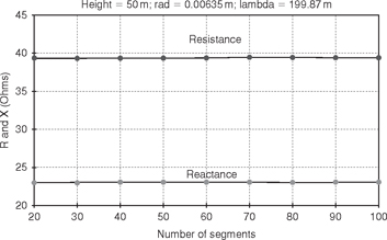
FIGURE 8-2(b)![]()
Segmentation on a thin wire.
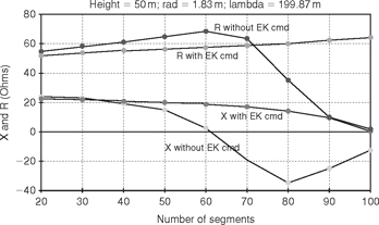
FIGURE 8-2(c)![]()
Segmentation on a thick wire.
As a final comment on this subject, it is worthwhile to know that the dependency of the calculated impedance on the ratio of Δ/a is imposed by the numerical solutions employed in NEC-2 and are not a physical characteristic of the tower proper. As mentioned earlier, NEC-2 results are close approximations rather than exact solutions. In this particular instance, using the EK command changes the assumption that the current flows as a thin filament on the wire axis to one that has the current flowing axially over the complete wire surface. The latter gives a more realistic solution but requires more computer effort, which is not a serious handicap to modern computers. It is important to recognize, however, that both processes involve assumptions and both have limitations.
8.2.2 Tower Diameter
Figure 8-3(a) shows the effect on drive point impedance when the tower diameter is varied. The plot for short towers (G = 54°) shows
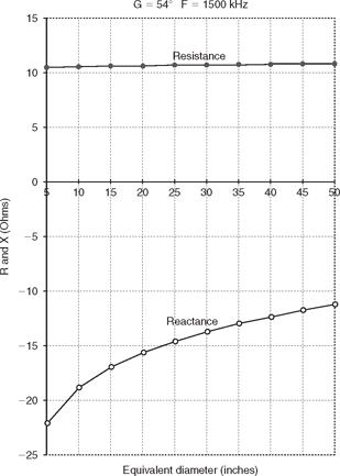
FIGURE 8-3(a)![]()
Impedance versus tower diameter: G = 54°.
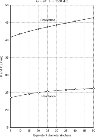
FIGURE 8-3(b)![]()
Impedance versus tower diameter: G = 90°.
very little change in the resistive component as diameter is varied but there is significant change in the reactive component. With the resistance remaining near constant and the reactance decreasing, the effective Q of the antenna decreases, resulting in an increased bandwidth. This supports the notion that “fat” antennas have a broader bandwidth.
At G = 90°, changing the tower diameter has only a minimal effect on drive point impedance but at the taller heights, changing tower diameter changes the drive point impedance significantly.

FIGURE 8-3(c)![]()
Impedance versus tower diameter: G = 126°.
Notice that at G = 126°, the reactive component of impedance decreases by approximately 50 percent as the tower diameter increases. At the same time, the resistive component rises almost 30 percent.
The change in the resistive component is even greater, albeit in the opposite direction, as the tower height climbs to 180°. The resistive component falls to less one-third its thin value and the reactive component reduces to two-thirds its thin value.
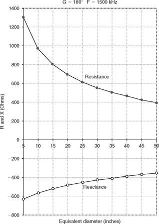
FIGURE 8-3(d)![]()
Impedance versus tower diameter: G = 180°.
Thus, it may be concluded that tower diameter is more significant for tall towers than it is for shorter ones.
8.2.3 Segment and Radius Taper
The GC command in the NEC-2 input file permits both the radius and the segment length to be tapered from one end of the wire to the
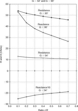
FIGURE 8-4(a)![]()
Impedance versus taper: G = 54° & G = 90°.
other. That this feature can be used as a matching tool is shown in Figure 8-4.
These figures show the effect of tapering the segment length over the tower height which has been divided into 20 segments with a ratio of (segment N length/segment N-1 length) = 1.1. In addition, the tower radius is tapered in 20 segments from a starting radius of R at the base of the tower to radius r at the top.
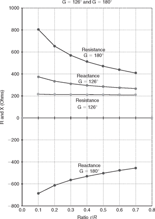
FIGURE 8-4(b)![]()
Impedance versus taper: G = 126° & G = 180°.
Again, the effect of this variation is rather minor for the short tower (G = 54°) but grows to be quite significant on the taller towers.
8.2.4 Base Capacity
The base insulator and the tower itself present an effective capacity from tower bottom to ground.
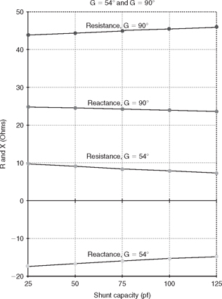
FIGURE 8-5(a)![]()
Impedance versus base capacity: G = 54° & G = 90°.
Figure 8-5 shows how this capacity affects drive point impedance. On the taller towers, it appears that it is almost a necessity that this capacity be included in the model. The shorter towers, G = 54° and G = 90°, in Figure 8-5(a) show almost no change as the base capacity varies from 25 pf to 125 pf. On the other hand, with G = 180° in Figure 8-5(b), the resistive component of the drive point impedance changes from more than 400 ohms to 200 ohms as the base capacity is increased from 25 pf to 125 pf.
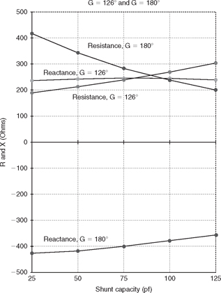
FIGURE 8-5(b)![]()
Impedance versus base capacity: G = 126° & G = 180°.
For all tower heights, the change in the reactive component of the base drive impedance is only small to moderate.
8.2.5 Drive Segment Radius
The drive segment is essentially a model of the base insulator in tower configurations shown in Figures 3-1(c), (d), and (e). As such, some latitude is permissible in defining the radius of that segment.
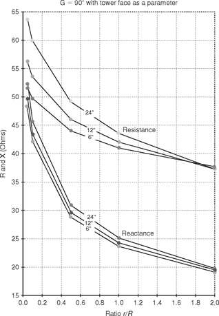
FIGURE 8-6(a)![]()
Impedance versus drive segment radius with tower face as a parameter: G = 90°.
Figure 8-6 shows impedance versus the drive segment radius (r) expressed as a ratio with the radius of the main radiator (R). And as it turns out, the nature of NEC-2 is such that the drive point impedance is quite sensitive to the radius of that segment. Unfortunately, it is not always possible to select a drive segment radius to simultaneously match both the measured resistance and reactance. It appears that shorter towers are more likely to match resistance and taller towers are more likely to match reactance.
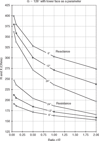
FIGURE 8-6(b)![]()
Impedance versus drive segment radius with tower face as a parameter: G = 126°.
8.3 Exercise
8-1. Using a triangular tower whose height is 66° with a 12″ face and operating at 1070 kHz with the configuration shown in Chapter 3, Figure 3-1(c), show how the calculated drive point impedance varies as the length of the drive segment is changed from 1 meter to 10 meters in 1-meter increments. The radius of the drive segment is 40 percent of the radius of the tower proper.