
“Surely it is not knowledge, but learning; not owning but earning; not being there, but getting there; that gives us the greatest pleasure.”
—Carl Friedrich Gauss, 1777–1855, Mathematician
I. CLASSIFICATION OF MATERIALS AND FLUID PROPERTIES
What is a fluid? It isn’t a solid, but what is a solid? Perhaps it is easier to define these materials in terms of how they respond (i.e., deform or flow) when subjected to an applied force in a specific situation, such as simple shear illustrated in Figure 3.1 (which is virtually identical to Figure 1.1). We envision the material contained between two large parallel plates of area Ay, the bottom one being fixed and the upper one subject to a tangential force Fx in the x direction. This force causes the upper plate to be displaced in the x direction by an amount Ux and/or to move with a constant velocity Vx after reaching a steady state.
The material is assumed to adhere to the plates (known as the “no-slip” condition), and its deformation properties can be classified by the way the top plate responds when the force is applied. The mechanical behavior of a material, and its corresponding mechanical or rheological* properties, can be defined in terms of how the shear stress (τyx) (force per unit area) and the shear strain (γyx) (which is a relative displacement and a measure of deformation) are related. These are defined, respectively, in terms of the total force (Fx) acting on area Ay of the plate and the relative displacement (Ux/hy) of the plates, that is,
(3.1) |
and
(3.2) |
The manner in which the shear strain, or displacement, responds to an applied shear stress, or force, (or vice versa) in this situation defines the mechanical or rheological characteristics of the material. The parameters in any quantitative functional relation between the stress and strain are the rheological properties of the material. It is noted that the shear stress has dimensions of force per unit area (with units of, e.g., Pa, dyn/cm2, or lbf/ft2) and that shear strain is dimensionless (it has no units).
For example, if the material between the plates is a perfectly rigid solid (e.g., a brick), it will not move at all, no matter how much force is applied (unless it breaks). Thus, the quantitative relation that defines the behavior of this material is
(3.3) |
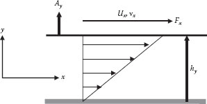
FIGURE 3.1 Simple shear.
However, if the top plate moves a distance that is in proportion to the applied force and then stops, the material is called a linear elastic (Hookean) solid (e.g., rubber). The quantitative relation that defines such a material is
(3.4) |
where G is a constant called the shear modulus. Note also that if the force (stress) is removed, the displacement (strain) also goes to zero, that is, the material reverts to its original undeformed state. Such an ideal elastic material is thus said to have a “perfect memory.”
On the other hand, if the top plate moves but its displacement is not directly proportional to the applied force (it may be either more or less than proportional to the force), the material is said to be a nonlinear (i.e., non-Hookean) elastic solid. It can be represented by an equation of the form
(3.5) |
Here, G is still called the shear modulus but it is no longer a constant. It is, instead, a function of either how far the plate moves (γyx) or the magnitude of the applied force (τyx), that is, G(γ) or G(τ). The particular form of the function will depend upon the specific nature of the material. Note, however, that such a material still exhibits a “perfect memory” because it returns to its undeformed state when the force (stress) is removed.
At the other extreme, if the molecules of the material are so far apart that they exert negligible attraction on each other (e.g., a gas under very low pressure), the plate can be moved by the application of a negligible force. The equation that describes this material is
(3.6) |
Such an ideal material is called an inviscid (Pascalian) fluid. However, if the molecules do exhibit a significant mutual attraction such that the force (e.g., the shear stress) is proportional to the relative rate of movement (i.e., the velocity gradient), the material is known as a Newtonian fluid. The equation that describes this behavior is
(3.7) |
where is the rate of shear strain, or shear rate for short:
(3.8) |
and μ is the fluid viscosity. Note that Equation 3.7 defines the viscosity, that is, , which has dimensions of Ft/L2 (with units of (Pa s), (dyn s/cm2 = gm/cm s = Poise), (lbf s/ft2), etc.).* Note that when the stress is removed from this fluid, the strain rate goes to zero, that is, the motion stops, but there is no “memory” or tendency to return to any past state.
If the properties of the fluid are such that the shear stress and shear rate are not directly proportional but are instead related by some more complex function, the fluid is said to be non-Newtonian (similar to a non-Hookean solid). For such fluids, the viscosity is still defined as , but it is no longer a constant, being instead a function of either the shear rate or shear stress. It is called the apparent viscosity (function) and is designated by η:
(3.9) |
The actual mathematical form of this function will depend upon the nature (i.e., the “constitution”) of the particular material. The most common fluids of simple structure (water, air, glycerin, oils, etc.) are Newtonian. However, fluids with complex structure (high-molecular-weight polymer melts or solutions, suspensions of fine particles, emulsions, foams, soap and surfactant solutions, etc.) are generally non-Newtonian. Some very common examples of non-Newtonian fluids are mud, paint, ink, mayonnaise, shaving cream, dough, mustard, yoghurt, catsup, toothpaste, blood, synovial fluid, sludge, etc.
Actually, some substances exhibit both elastic (solid) properties and viscous (fluid) properties under appropriate conditions. For instance, a ball made from silly putty bounces off the floor like a rubber ball (i.e., elastic), whereas when left alone it relaxes into a “puddle” on its own over a long time scale (i.e., viscous). These materials are said to be viscoelastic and are most notably materials composed of high-molecular-weight polymers and/or complex molecular structure. The complete description of the rheological properties of these materials may involve a function relating the stress and strain as well as derivatives or integrals of these with respect to time. Because the elastic properties of these materials (both fluids and solids) impart “memory” to the material (as described previously), which results in a tendency to recover to a preferred state upon the removal of the force (stress), they are often termed “memory materials” and exhibit time-dependent properties.
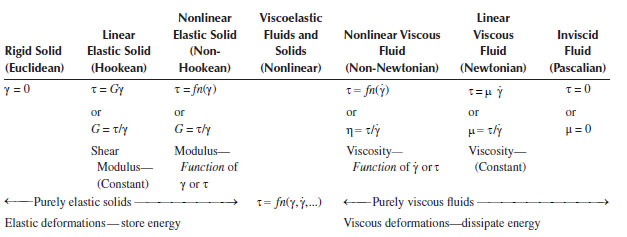
This classification of material behavior is summarized in Table 3.1 (in which the subscripts (x, y) have been omitted for simplicity). Since we are concerned with fluids, we will concentrate primarily on the flow behavior of Newtonian and non-Newtonian fluids. However, we will later illustrate some of the unique characteristics of viscoelastic fluids, such as the ability of solutions of certain high polymers to flow through pipes in turbulent flow with much less energy expenditure than the solvent alone (see Section VIII of Chapter 6).
II. DETERMINATION OF FLUID VISCOUS (RHEOLOGICAL) PROPERTIES
As previously discussed, the flow behavior of fluids is determined by their rheological properties, which govern the relationships between shear stress and shear rate. In principle, these properties could be determined by measurements in a “simple shear” test as illustrated in Figure 3.1. One would put the “unknown fluid” in the gap between the plates, subject the upper plate to a specified velocity (V), and measure the required force (F) (or vice versa). The shear stress (τ) would be determined by F/A, the shear rate () is given by V/h, and the viscosity (η) by .
The experiment is repeated for different combinations of V and F to determine the viscosity at various shear rates (or shear stresses). However, this geometry is not convenient to work with, because it is hard to keep the fluid in the gap with no confining walls, and correction for the effect of the walls is not simple. However, there are more convenient geometries for measuring viscous properties, as described in the following sections. The working equations used to obtain viscosity from measured quantities will be given here, although the development of these equations will be delayed until after the appropriate fundamental principles have been discussed.
Classification of Materials
Source: Darby, R., Viscoelastic Fluids, Marcel Dekker, New York, 1976.
A. CUP AND BOB (COUETTE) VISCOMETER
As the name implies, the cup and bob (Couette) viscometer consists of two concentric cylinders, the outer “cup” and the inner “bob,” with the test fluid in the annular gap (see Figure 3.2).
One cylinder (preferably the cup) is rotated at a fixed angular velocity (Ω). The force is transmitted to the sample causing it to deform and is then transferred by the fluid to the other cylinder (i.e., the bob). This force results in a torque (T) that can be measured by a torsion spring, for example. Thus, the known quantities are the radius of the inner bob (Ri) and the outer cup (Ro), the length of bob surface in contact with the fluid sample (L), and the measured angular velocity (Ω) and torque (T). From these quantities, we must determine the corresponding shear stress and shear rate to find the fluid viscosity. The shear stress is determined by a balance of moments on a cylindrical surface within the sample (at a distance r from the center), and the torsion spring
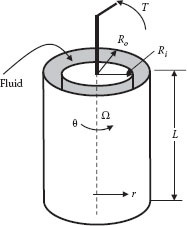
FIGURE 3.2 Cup and bob (Couette) viscometer.
or
(3.10) |
where the subscripts on the shear stress (r, θ) represent the force in the θ direction acting on the r surface (the cylindrical surface perpendicular to r). Solving for the shear stress:
(3.11) |
Setting r = Ri gives the stress on the bob surface (τi), and r = Ro gives the stress on the cup (τo). If the gap is small [i.e., (Ro − Ri)/Ri ≤ 0.02], the curvature can be neglected and the flow in the gap is equivalent to the flow between flat parallel plates, similar to that shown in Figure 3.1. In this case, an average shear stress should be used [i.e., (τi+τo)/2], and the average shear rate is given by
or
(3.12) |
where β = Ri/Ro. However, if the gap is not small, the shear rate must be corrected for the curvature in the velocity profile. This can be done by applying the following approximate expression for the shear rate at the bob (which is accurate to ±1% for most conditions and is better than ±5% for the worst case; see, e.g., Darby, 1985):
(3.13) |
where
(3.14) |
is the point slope of the plot of log T versus log Ω, at the value of Ω (or T) in Equation 3.12. Thus, a series of data points of T versus Ω must be obtained in order to determine the value of the slope (n′) at each point, which is needed to determine the corresponding values of the shear rate. If n′ = 1 (i.e., T ∝ Ω), the fluid is Newtonian. The viscosity at each shear rate (or shear stress) is then determined by dividing the shear stress at the bob (Equation 3.11 with r = Ri) by the shear rate at the bob (Equation 3.13), for each data point.
Example 3.1
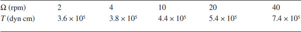
The following data were taken in a cup and bob viscometer, with a bob radius of 2 cm, a cup radius of 2.05 cm, and a bob length of 15 cm. Determine the viscosity of the sample, and the equation for the model that best represents this viscosity.
Torque, T (dyn cm) |
Speed, Ω (rpm) |
2,000 |
2 |
3,500 |
4 |
7,200 |
10 |
12,500 |
20 |
20,000 |
40 |
The viscosity is the shear stress at the bob, as given by Equation 3.11, divided by the shear rate at the bob, as given by Equation 3.13.
Sample Calculation:
For the first data point, the shear stress at the bob is given by
and the shear rate is given by Equation 3.13. The value of β for this system is β = 2.0/2.05 = 0.976. Although this is a small gap, we will assume it is not small enough to use Equation 3.12 for the shear rate and will illustrate the use of Equation 3.13 instead. The value of n′ in Equation 3.13 is determined from the point slope of the (log T) versus (log rpm) plot at each data point, as illustrated by the plot shown in Figure E3.1. The line through the data is the best fit of all data points by linear least squares (this is easily found by using a spreadsheet) and is found to have a slope of 0.77 (with r2 = 0.999). In general, if the data do not fall on a straight line as in this example, the point slope (tangent) must be determined at each data point, resulting in a different value of n′ for each data point. Using 0.77 for n′ in Equation 3.13 gives
Shear Stress at Bob (dyn/cm2) |
Shear Rate at Bob (s−1) |
Viscosity (Poise) |
5.31 |
8.90 |
0.61 |
9.28 |
17.8 |
0.53 |
19.1 |
44.5 |
0.43 |
33.2 |
89.0 |
0.37 |
53.1 |
178 |
0.31 |
The plot of viscosity versus shear rate for this material is shown in Figure E3.1b.
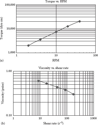
FIGURE E3.1 Examples of (a) torque versus speed and (b) the corresponding calculated viscosity versus shear rate for data in Example 3.1.
It should be noted that in practice some corrections arising from the edge effects (or end effects), secondary flows (Taylor vortices) at high rotational speeds, etc. may be required depending upon the specific designs of cup and bob viscometers and the properties of the fluid. These aspects are described in detail in Darby (1976) and Chhabra and Richardson (2008) and generally limit the maximum reliable shear rate attainable in cup and bob viscometers.
B. TUBE FLOW (POISEUILLE) VISCOMETER
Another common method of determining viscosity is by measuring the total driving force or “pressure drop” (ΔΦ = ΔP + ρgΔz) and flow rate (Q) in steady laminar flow through a straight, uniform circular tube of length L and diameter D (this is called Poiseuille flow). This can be done by using pressure taps through the tube wall to measure the pressure difference directly or by measuring the total pressure difference from a reservoir to the end of the tube, as illustrated in Figure 3.3. The latter is more common because tubes of very small diameter are usually used, but this arrangement requires that correction factors be applied for the static head of the fluid in the reservoir and the entrance pressure loss from the reservoir to the tube (detailed descriptions of the relevant corrections can be found in Darby (1976) and Chhabra and Richardson (2008)). As will be shown later, a momentum (force) balance on the fluid in the tube provides a relation between the shear stress at the tube wall (τw) and the measured pressure drop:
(3.15) |
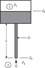
FIGURE 3.3 Tube flow (Poiseuille) viscometer.
where ΔΦ = Φ2 – Φ1 = (P2 − P1) +ρg (z2 − z1) is the net driving force from point 1 in the reservoir (at the surface of the liquid) to point 2 at the tube exit (corrected for the “entrance loss” from the reservoir to the tube (see Section III of Chapter 7). The diameter of the reservoir is normally much larger than that of the tube, so that the change in the head and the kinetic energy of the fluid in the reservoir can be neglected. The corresponding shear rate at the tube wall is given by
(3.16) |
where
(3.17) |
is the wall shear rate for a Newtonian (n′ = 1) fluid, and
(3.18) |
is the point slope of the log–log plot of ΔΦ versus Q, evaluated at each data point. This n′ is the same as that determined from the cup and bob viscometer, for a given fluid. As before, if n′ = 1 (i.e., ΔΦ∝ Q), the fluid is Newtonian. The apparent viscosity is given by .
Example 3.2
The following data were obtained for a 5% aqueous polymer solution in a horizontal pipe of 42 mm internal diameter. The pressure difference was measured by two pressure transducers mounted 63 cm apart in the middle section of the pipe so that end effects are negligible.

Obtain the true shear stress–shear rate data for this polymer solution.
Sample Calculation:
The values of Γ are calculated from Equation 3.17. For the first data point, the calculation is
625 |
104 |
714 |
1.47 |
564 |
100 |
643 |
1.56 |
488 |
90.7 |
557 |
1.63 |
383 |
80.0 |
437 |
1.83 |
343 |
72.0 |
391 |
1.84 |
272 |
62.3 |
310 |
2.00 |
219 |
54.2 |
250 |
2.17 |
187 |
49.3 |
213 |
2.31 |
147 |
42.2 |
167 |
2.52 |
114 |
36 |
130 |
2.77 |
66.7 |
25.5 |
76 |
2.36 |
As the tube in this case is horizontal, the driving force is simply the pressure difference, −ΔΦ = −ΔP, so the wall shear stress becomes
In order to evaluate the point slope, n′ = dlogτw/dlog(8V/D), these data are plotted in Figure E3.2 on log–log coordinates. The value of the slope of the plot, n′, is seen to be constant at n′ = 0.64. Therefore, the true shear rate at the wall can be calculated using Equation 3.16:
and the apparent viscosity at this shear rate is
These values are also summarized in the preceding table. The viscosity versus shear rate curve is also shown in Figure E3.2, where this olymer solution is seen to exhibit shear thinning behavior.
III. TYPES OF NON-NEWTONIAN FLUID BEHAVIOR
When the measured values of shear stress or viscosity are plotted versus shear rate, various types of behavior may be observed depending upon the fluid properties, as shown in Figures 3.4 and 3.5. It should be noted that the shear stress and shear rate can both be either positive or negative, depending upon the direction of motion or the applied force, the reference frame, etc. (however, by our convention, they are always of the same sign). Because the viscosity must always be positive, the shear rate (or shear stress) argument in the viscosity function for a non-Newtonian fluid should be the absolute magnitude regardless of the actual sign of the shear rate and shear stress.
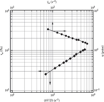
FIGURE E3.2. Plot of τw versus Γ(8V/D) to evaluate n′ and viscosity versus shear rate.
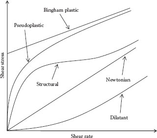
FIGURE 3.4 Shear stress versus shear rate for various types of fluid behavior.
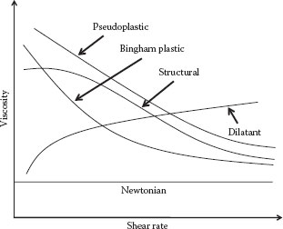
FIGURE 3.5 Viscosity versus shear rate for fluids in Figure 3.4.
If the shear stress versus shear rate plot is a straight line through the origin (or a straight line with a slope of unity on a log–log plot), the fluid is Newtonian:
(3.19) |
where μ is the viscosity.
If the data appear to be linear but do not extrapolate through the origin, intersecting the shear stress (τ) axis instead at a shear stress value of τo, the material is called a Bingham plastic:
(3.20) |
The yield stress,τo, and the high shear limiting (or plastic) viscosity, μ∞, are the two rheological properties required to determine the flow behavior of a Bingham plastic. The positive sign is used when τ and are positive, and the negative sign when they are negative. The viscosity function for the Bingham plastic is
(3.21) |
or
(3.22) |
Because this material will not flow unless the shear stress exceeds the yield stress, these equations apply only when |τ| >τo. For smaller values of the shear stress, the material behaves as a rigid solid, that is,
(3.23) |
As is evident from Equation 3.21 or 3.22, the Bingham plastic exhibits a shear thinning viscosity, that is, the larger the shear stress or shear rate, the lower the viscosity. This behavior is typical of many concentrated slurries and suspensions such as muds, paints, foams, emulsions (e.g., mayonnaise), ketchup, or blood.
If the data (either shear stress or viscosity) exhibit a straight line on a log–log plot, the fluid is said to follow the power law model, which can be represented as
(3.24) |
The two viscous rheological properties are m, the consistency coefficient, and n, the flow index. The apparent viscosity function for the power law model in terms of shear rate is
(3.25) |
or in terms of shear stress
(3.26) |
Note that n is dimensionless but m has dimensions of Ftn/L2. However, m is also equal to the apparent viscosity of the fluid at a shear rate of 1 s−1, so it is a “viscosity” parameter with equivalent units. It is evident that if n = 1 the power law model reduces to a Newtonian fluid with m = μ. If n < 1, the fluid is shear thinning (or pseudoplastic), and if n > 1 the model represents shear thickening (or dilatant) behavior, as illustrated in Figures 3.5 and 3.6. Most non-Newtonian fluids are shear thinning, whereas shear thickening behavior is relatively rare, being observed primarily for some concentrated suspensions of very small particles (e.g., starch suspensions) and some unusual polymeric fluids. The power law model is very popular for curve fitting viscosity data for many fluids over one to three decades of shear rate. However, it is dangerous to extrapolate beyond the range of measurements using this model, because for n < 1 it predicts a viscosity that increases without bound as the shear rate decreases and a viscosity that decreases without bound as the shear rate increases, both of which are physically unrealistic.
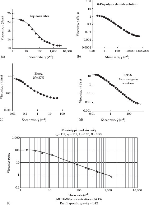
FIGURE 3.6 (a–e) Some examples of structural viscosity behavior for a range of fluids.
D. STRUCTURAL VISCOSITY MODELS
The typical viscous behavior for many non-Newtonian fluids (e.g., polymeric fluids, flocculated suspensions, colloids, foams, gels) is illustrated by the curves labeled “structural” in Figures 3.5 and 3.6. These fluids exhibit Newtonian behavior at very low and very high shear rates, with shear thinning or pseudoplastic behavior at intermediate shear rates. In some materials, this can be attributed to a reversible “structure” or network that forms in the “rest” or equilibrium state. When the material is sheared, the structure breaks down, resulting in a shear-dependent (shear thinning) behavior. Some real examples of this type of behavior are shown in Figure 3.6. These show that structural viscosity behavior is exhibited by fluids as diverse as polymer solutions, blood, latex emulsions, and mud (sediment). Equations (i.e., models) that represent this type of behavior are described in the following sections.
The Carreau model (Carreau, 1972) is very useful for describing the viscosity of structural fluids:
(3.27) |
This model contains four rheological parameters: the low shear limiting viscosity (ηo), the high shear limiting viscosity (η∞), a time constant (λ), and the shear thinning index (p). This is a very general viscosity model, and it can represent the viscosity function for a wide variety of materials. However, it may require data over a range of six to eight decades of shear rate to completely define the shape of the curve (and hence to determine all four parameters). As an example, Figure 3.7 shows viscosity data for several polyacrylamide solutions over a range of about six orders of magnitude of shear rate, with the curves through the data points representing the Carreau model fit to the data. The corresponding values of the Carreau parameters for each of the curves are given in Table 3.2. In fact, over certain ranges of shear rate, the Carreau model reduces to various other popular models for special cases (including the Bingham plastic and power law models), as shown below.
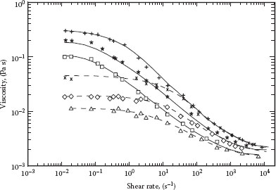
FIGURE 3.7 Viscosity data and Carreau model fit of polyacrylamide solutions. (From Darby, R. and Pvisa-Art, S., Can. J. Chem. Eng., 69, 1395, 1991.)
Values of Carreau Parameters for Model Fit in Figure 3.7
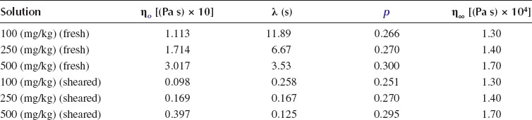
Source: Darby, R. and Pvisa-Art, S., Can. J. Chem. Eng., 69, 1395, 1991.
a. Low to Intermediate Shear Rate Range
If η∞ ≪ (η, ηo), the Carreau model reduces to a three-parameter model (ηo, λ, and p) that is equivalent to a power law model with a low shear limiting viscosity of ηo, also known as the Ellis model, which can be written as follows:
(3.28) |
b. Intermediate to High Shear Rate Range
If ηo≫(η, η∞) and , the Carreau model reduces to the equivalent of a power law model with a high shear limiting viscosity, called the Sisko model:
(3.29) |
Although this appears to have four parameters, it is really a three-parameter model because the combination ηo/λ2p is a single parameter, along with the two parameters p and η∞.
c. Intermediate Shear Rate Behavior
For η∞ ≪ η ≪ ηo and , the Carreau model reduces to the power law model:
(3.30) |
In this case, the power law parameters m and n are equivalent to the following combinations of Carreau parameters:
(3.31) |
d. Bingham Plastic Behavior
If the value of p is set equal to 1/2 in the Sisko model, the result is equivalent to the Bingham plastic model:
(3.32) |
where
the yield stress τo is equivalent to ηo/λ
η∞ is the limiting (high shear) viscosity
A variety of more complex models have been proposed to fit a wider range and variety of viscosity data. Three of these are presented here.
a. Meter Model
A stress-dependent viscosity model, which has the same general characteristics as the Carreau model except that it uses shear stress as the independent variable, is the Meter model (Meter, 1964):
(3.33) |
where
σ is a characteristic stress parameter
a is the shear thinning index
This form is particularly suited for conditions when the shear stress is known.
b. Yasuda Model
The Yasuda model (Yasuda et al., 1981) is a modification of the Carreau model with one additional parameter a (a total of five parameters):
(3.34) |
which reduces to the Carreau model for a = 1 (this is also sometimes called the Carreau–Yasuda model). This model is particularly useful for representing melt viscosity data for polymers with a broad molecular weight distribution, for which the zero-shear viscosity is approached very gradually. Both of these models reduce to Newtonian behavior at very low and very high shear rates and to power law behavior at intermediate shear rates.
IV. TEMPERATURE DEPENDENCE OF VISCOSITY
All fluid properties are dependent upon temperature. For most fluids, the viscosity is the property that is most sensitive to temperature changes. The following relations apply to Newtonian fluids, although for non-Newtonian fluids represented by any of the above models, any model parameter having dimensions of viscosity will generally follow similar temperature dependence.
For liquids, as the temperature increases the degree of molecular motion increases, reducing the short-range attractive forces between molecules and thereby lowering the viscosity of the fluid. The viscosity of various liquids is shown as a function of temperature in Appendix A. For many liquids, this temperature dependence can be represented reasonably well by the Arrhenius equation:
(3.35) |
where T is the absolute temperature. If the viscosity of a liquid is known at two different temperatures, this information can be used to evaluate the parameters A and B, which then permits the calculation of the viscosity at any other temperature. If the viscosity is known at only one temperature, this value can be used as a reference point to establish the temperature scale for Figure A.2, which can then be used to estimate the viscosity at any other temperature. Viscosity data for a large number of Newtonian liquids have been fitted by Yaws et al. (1994) by the equation
(3.36) |
where
T is in Kelvin
the viscosity μ is in centipoise
The values of the correlation parameters A, B, C, and D are tabulated by Yaws et al. (1994).
For non-Newtonian fluids, any model parameter with the dimensions or physical significance of viscosity (e.g., the power law consistency, m, or the Carreau parameters η∞ and ηo) will depend on temperature in a manner similar to the viscosity of a Newtonian fluid (e.g., Equation 3.35 or 3.36).
In contrast to the behavior of liquids, the viscosity of a gas increases with increasing temperature. This is because gas molecules are much farther apart, so the short-range attractive forces are very small. However, as the temperature is increased, the molecular kinetic energy increases, resulting in a greater exchange of momentum between the molecules and consequently resulting in a higher viscosity. The viscosity of gases is not as sensitive to temperature as that of liquids, however, and can often be represented by the equation
(3.37) |
The parameters a and b can be evaluated from a knowledge of the viscosity at two different temperatures, and the equation can then be used to calculate the viscosity at any other temperature. The value of the parameter b is often close to 1.5. In fact, if the viscosity (μ1) of a gas is known at only one temperature (T1), the following equation can be used to estimate the viscosity at any other temperature:
(3.38) |
where
the temperatures are in Rankine
TB is the boiling point of the gas
In contrast to viscosity, the density of both liquids and gases decreases with increasing temperature, and the density of gases is much more sensitive to temperature than that of liquids. If the density of a liquid (ρ) and its vapor (ρv) are known at 60°F, the density at any other temperature can be estimated by the equation
(3.39) |
where
the temperatures are in degrees Rankine
Tc is the critical temperature of the substance
The value of N is given in Table 3.3 for various liquids. This method yields the value of (ρ – ρv)T at the temperature of interest (T) and one must still estimate the value of ρv to evaluate the density of the liquid, ρ.
The specific gravity of hydrocarbon liquids at 60°F is also often represented by the API gravity, or °API:
(3.40) |
For gases, if the temperature is well above the critical temperature and the pressure below the critical pressure, the ideal gas law usually applies:
(3.41) |
where
M is the gas molecular weight
Temperatures and pressures are absolute
is the standard molar volume (22.4 m3/(kg mol) at 273 K and 1 atm, 359ft3/(lb mol) at 492°R and 1 atm, or 379.4ft3/lb mol at 520°R (60°F) and 1 atm)
The notation SCF (which stands for “standard cubic feet”) is often used for hydrocarbon gases to represent the volume in ft3 that would be occupied by the gas at 60°F and 1 atm pressure and is thus actually a measure of the mass of the gas.
For other methods of predicting fluid properties and their temperature dependence, the reader is referred to the book by Reid et al. (1977).
Parameter N in Equation 3.39
Liquid |
N |
Water and alcohols |
4 |
Hydrocarbons and ethers |
3.45 |
Organics |
3.23 |
Inorganics |
3.03 |
Surface tension is a physical property of an interface between two phases such as a liquid–liquid, liquid–gas, or liquid–solid interface. The unique orientation of the fluid molecules at such an interface gives rise to unique forces and energy at the interface. For instance, it is the surface tension of water that tends to keep the small air bubbles spherical! Similarly, it is the surface tension that makes the flow of oil in narrow pores and passages of the rocks rather difficult. Surface tension arises from the cohesion between molecules at the fluid interface. A molecule surrounded by identical molecules experiences a zero net force, as it is pulled equally in all directions. In contrast, a molecule close to a wall, or an interface with another fluid, experiences a net force due to this orientation. From a fluid mechanics standpoint, surface tension can complicate the analysis of problems involving the formation and/or motion of bubbles and drops in another liquid such as in ink-jet printers, or when the flow passage is of the order of micro- and nanometers such as in microfluidic devices. In contrast to the forces such as pressure or shear stresses that act on areas and the body forces acting on the volume of a fluid, surface tension is a force per unit length of the interface with the units of dyn/cm or N/m. Note that surface tension also represents a concentration of surface energy, with dimensions of energy/area (e.g., N m/m2). Thus, in microfluidic and nanodevices, the characteristic dimension (l) is of the order of micrometers or nanometers and the corresponding surface areas and volumes are O (l2) and O (l3), respectively. Thus, in such situations, the surface tension force can be a significant factor. Finally, there are situations when the driving force for the flow arises from the surface tension gradient itself, such as the flow in capillaries. While none of these situations are addressed in depth in this text, in view of the growing importance of nano- and microscale engineering, the readers must be aware of these issues and one must look up specialized books on this subject (e.g., Probstein, 2003).
The key points covered in this chapter include:
• The understanding and description of linear and nonlinear deformation and flow of solids and fluids.
• The measurement of fluid viscous properties by Couette and Poiseuille viscometers.
• The types of fluid materials that exhibit nonlinear viscous (non-Newtonian) behavior.
• The various mathematical models that are capable of describing different classes of non- Newtonian behavior.
• Temperature dependency of the viscosity of liquids and gases.
• Nature of the temperature dependency of density for liquids and gases.
• Awareness of the importance of surface tension in systems of small dimensions.
RHEOLOGICAL PROPERTIES
1.
(a) Using tabulated data for the viscosity of water and SAE 10 lube oil as a function of temperature, plot the data in a form that is consistent with each of the following equations:
(i) μ = A exp(B/T)
(ii) μ = aTb
(b) Arrange the equations in (a) in such a form that you can use linear regression analysis to determine the values of A, B and a, b that give the best fit to the data for each fluid (a spreadsheet is useful for this). (Note that T is the absolute temperature here.)
2. The viscosity of a fluid sample is measured in a cup and bob viscometer. The bob is 15 cm long with a diameter of 9.8 cm, and the cup has a diameter of 10 cm. The cup rotates, and the torque is measured on the bob. The following data were obtained:
(a) Determine the viscosity of the sample.
(b) What viscosity model equation would be the most appropriate for describing the viscosity of this sample? Convert the data to corresponding values of viscosity versus shear rate, and plot them on appropriate axes consistent with the data and your equation. Use linear regression analysis in a form that is consistent with the plot to determine the values of each of the parameters in your equation.
(c) What is the viscosity of this sample at a cup speed of 100 rpm in the viscometer?
3. A fluid sample is contained between two parallel plates separated by a distance of 2 ± 0.1 mm. The area of the plates is 100 ± 0.01 cm2. The bottom plate is stationary, and the top plate moves with a velocity of 1 cm/s when a force of 315 ± 25 dyn is applied to it, and at 5 cm/s when the force is 1650 ± 25 dyn.
(a) Is the fluid Newtonian?
(b) What is its viscosity?
(c) What is the range of uncertainty to your answer to (b)?
4. The following materials exhibit flow properties that can be described by models that include a yield stress (e.g., Bingham plastic): (a) catsup, (b) toothpaste, (c) paint, (d) coal slurries, and (e) printing ink. In terms of typical applications of these materials, describe how the yield stress is beneficial to their behavior, in contrast to how they would behave if they were Newtonian.
5. Consider each of the fluids for which the viscosity is shown in Figure 3.7, all of which exhibit a “structural viscosity” characteristic. Explain how the “structure” of each of these fluids influences the nature of the viscosity curve for that fluid.
6. Starting with the equations for that define the power law and Bingham plastic fluids, derive the equations for the viscosity functions for these models as a function of shear stress, that is, η = fn (τ).
7. A paint sample is tested in a Couette (cup and bob) viscometer that has an outer radius of 5 cm, an inner radius of 4.9 cm, and a bob length of 10 cm. When the outer cylinder is rotated at a speed of 4 rpm, the torque on the bob is 0.0151 N m, and at a speed of 20 rpm, the torque is 0.0226 N m.
(a) What are the corresponding values of shear stress and shear rate for these two data points (in cgs units)?
(b) What can you conclude about the viscous properties of the paint sample?
(c) Which of the following models could be used to describe the paint:
(i) Newtonian
(ii) Bingham plastic
(iii) Power law?
Explain why.
(d) Determine the values of the fluid properties (i.e., parameters) of the models in (c) that could be used.
(e) What would the viscosity of the paint be at a shear rate of 500 s−1 (in poise)?
8. The quantities that are measured in a cup and bob viscometer are the rotation rate of the cup (rpm) and the corresponding torque transmitted to the bob. These quantities are then converted to corresponding values of shear rate () and shear stress (τ), which in turn can be converted to corresponding values of viscosity (η).
(a) Show what a log–log plot of τ versus g and η versus g would look like for materials that follow the following models: (i) Newtonian, (ii) power law (shear thinning), (iii) power law (shear thickening), (iv) Bingham plastic, and (v) structural.
(b) Show how the values of the parameters for each of the models listed in (a) can be evaluated from the respective plot of η versus . That is, relate each model parameter to some characteristic or combination of characteristics of the plot such as the slope, specific values read from the plot, intersection of tangent lines, etc.
9. What is the difference between shear stress and momentum flux? How are they related? Illustrate each one in terms of the angular flow in the gap in a cup and bob viscometer, in which the outer cylinder (cup) is rotated and the torque is measured at the stationary inner cylinder (bob).
10. A fluid is contained in the annulus in a cup and bob viscometer. The bob has a radius of 50 mm and a length of 10 cm and is made to rotate inside the cup by application of a torque on a shaft attached to the bob. If the cup inside radius is 52 mm and the applied torque is 0.03 ft lbf, what is the shear stress in the fluid at the bob surface and at the cup surface? If the fluid is Newtonian with a viscosity of 50 cP, how fast will the bob rotate (in rpm) with this applied torque?
11. You measure the viscosity of a fluid sample in a cup and bob viscometer. The radius of the cup is 2 in. and that of the bob is 1.75 in., and the length of the bob is 3 in. At a speed of 10 rpm, the measured torque is 500 dyn cm, and at 50 rpm, it is 1200 dyn cm. What is the viscosity of the fluid? What can you deduce about the properties of the fluid?
12. A sample of coal slurry is tested in a Couette (cup and bob) viscometer. The bob has a diameter of 10.0 cm and a length of 8.0 cm, and the cup has a diameter of 10.2 cm. When the cup is rotated at a rate of 2 rpm, the torque on the bob is 6.75 × 10⁴ dyn cm, and at a rate of 50 rpm, it is 2.44 × 10⁶ dyn cm. If the slurry follows the power law model, what are the values of the flow index and consistency coefficient? If the slurry follows the Bingham plastic model, what are the values of the yield stress and the limiting viscosity? What would the viscosity of this slurry be at a shear rate of 500 s−1 as predicted by each of these models? Which number would you be more likely to believe, and why?
13. You must analyze the viscous properties of blood. Its measured viscosity is 6.49 cP at a shear rate of 10 s−1 and 4.66 cP at a shear rate of 80 s−1.
(a) How would you describe these viscous properties?
(b) If the blood is subjected to a shear stress of 50 dyn/cm2, what would its viscosity be if it is described by (i) the power law model and (ii) the Bingham plastic model? Which answer do you think would be better, and why?
14. The following data were measured for the viscosity of a 500 ppm polyacrylamide solution in distilled water:
Shear Rate (s−1) |
Viscosity (cP) |
Shear Rate (s−1) |
Viscosity (cP) |
0.015 |
300 |
15 |
30 |
0.02 |
290 |
40 |
22 |
0.05 |
280 |
80 |
15 |
0.08 |
270 |
120 |
11 |
0.12 |
260 |
200 |
8 |
0.3 |
200 |
350 |
6 |
0.4 |
190 |
700 |
5 |
0.8 |
180 |
2,000 |
3.3 |
2 |
100 |
4,500 |
2.2 |
3.5 |
80 |
7,000 |
2.1 |
8 |
50 |
20,000 |
2 |
Find the model that best represents these data, and determine the values of the model parameters by fitting the model to the data. (This can be done most easily by trial and error, using a spreadsheet.)
15. What viscosity model best represents the following data? Determine the values of the parameters in the model. Show a plot of the data together with the line that represents the model, to show how well the model works. (Hint: The easiest way to do this is by trial and error, fitting the model equation to the data using a spreadsheet.)
Shear Rate (s−1) |
Viscosity (Poise) |
0.007 |
7745 |
0.01 |
7690 |
0.02 |
7399 |
0.05 |
6187 |
0.07 |
5488 |
0.1 |
4705 |
0.2 |
3329 |
0.5 |
2033 |
0.7 |
1692 |
1 |
1392 |
2 |
952 |
5 |
576 |
7 |
479 |
10 |
394 |
20 |
270 |
50 |
164 |
100 |
113 |
200 |
77.9 |
500 |
48.1 |
700 |
40.4 |
1,000 |
33.6 |
2,000 |
23.8 |
5,000 |
15.3 |
7,000 |
13.2 |
10,000 |
11.3 |
20,000 |
8.5 |
50,000 |
6.1 |
100,000 |
5.5 |
16. You would like to determine the pressure drop in a slurry pipeline. To do this, you need to know the rheological properties of the slurry. To evaluate these properties, you test the slurry by pumping it through a 1/8 in. ID tube that is 10 ft long. You find that it takes a 5 psi pressure drop to produce a flow rate of 100 cm3/s in the tube and that a pressure drop of 10 psi results in a flow rate of 300 cm3/s. What can you deduce about the rheological characteristics of the slurry from these data? If it is assumed that the slurry can be adequately described by the power law model, what would be the values of the appropriate fluid properties (i.e., the flow index and consistency parameter) for the slurry?
17. A film of paint, 3 mm thick, is applied to a flat surface that is inclined to the horizontal by an angle θ. If the paint is a Bingham plastic, with a yield stress of 150 dyn/cm2, a limiting viscosity of 65 cP, and a SG of 1.3, how large would the angle θ have to be before the paint would start to run? At this angle, what would the shear rate be if the paint follows the power law model instead, with a flow index of 0.6 and a consistency coefficient of 215 (in cgs units)?
18. A thick suspension is tested in a Couette (cup and bob) viscometer that has a cup radius of 2.05 cm, a bob radius of 2.00 cm, and a bob length of 15 cm. The following data are obtained:
Cup Speed (rpm) |
Torque on Bob (dyn cm) |
2 |
2,000 |
4 |
6,000 |
10 |
19,000 |
20 |
50,000 |
50 |
150,000 |
What can you deduce about (a) the viscous properties of this material, and (b) the best model to use to represent these data?
19. You have obtained data for a viscous fluid in a cup and bob viscometer that has the following dimensions: cup radius = 2 cm, bob radius = 1.5 cm, bob length = 3 cm. The data are tabulated in the following, where n′ is the point slope of the log T versus log N curve:
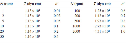
(a) Determine the viscosity of the fluid. How would you describe its viscosity?
(b) What kind of viscous model (equation) would be appropriate to describe this fluid?
(c) Use the data to determine the values of the fluid properties that are defined by the model.
20. A sample of a viscous fluid is tested in a cup and bob viscometer that has a cup radius of 2.1 cm, a bob radius of 2.0 cm, and a bob length of 5 cm. When the cup is rotated at 10 rpm, the torque measured at the bob is 6,000 dyn cm, and at 100 rpm, the torque is 15,000 dyn cm.
(a) What is the viscosity of this sample?
(b) What can you conclude about the viscous properties of the sample?
(c) If the cup is rotated at 500 rpm, what will be the torque on the bob and the fluid viscosity? Clearly explain any assumptions you make to answer this question, and tell how you might check the validity of these assumptions.
21. You have a sample of a sediment that is non-Newtonian. You measure its viscosity in a cup and bob viscometer having a cup radius of 3.0 cm, a bob radius of 2.5 cm, and a length of 5 cm. At a rotational speed of 10 rpm, the torque transmitted to the bob is 700 dyn cm, and at 100 rpm, the torque is 2500 dyn cm.
(a) What is the viscosity of the sample?
(b) Determine the values of the model parameters that represent the sediment viscous properties if it is represented by (i) the power law model or (ii) the Bingham plastic model.
(c) What would the flow rate of the sediment be (in cm3/s) in a 2 cm diameter tube, 50 m long, that is subjected to a differential pressure driving force of 25 psi assuming that (i) the power law model and (ii) the Bingham plastic model apply?
Which of these two answers do you think is best, and why?
22. Acrylic latex paint can be described by the Bingham plastic model with a yield stress of 112 dyn/cm2, a limiting viscosity of 80 cP, and a density of 0.95 g/cm3. What is the maximum thickness of this paint that can be applied to a vertical wall without it running?
23. Santa Claus and his loaded sleigh are sitting on your roof, which is covered with snow. The sled’s two runners each have a length L and width W, and the roof is inclined at an angle θ to the horizontal. The thickness of the snow between the runners and the roof is H. If the snow has properties of a Bingham plastic, derive an expression for the total mass (m) of the loaded sleigh at which it will just start to slide on the roof if it is pointed straight downhill. If the actual mass is twice this minimum mass, determine an expression for the speed at which the sled will slide. (Note: Snow does not actually behave as a Bingham plastic!)
24. You must design a piping system to handle a sludge waste product. However, you don’t know the properties of the sludge, so you test it in a cup and bob viscometer with a cup diameter of 10 cm, a bob diameter of 9.8 cm, and a bob length of 8 cm. When the cup is rotated at 2 rpm, the torque on the bob is 2.4 × 10⁴ dyn cm, and at 20 rpm, it is 6.5 × 10⁴ dyn cm.
(a) If you use the power law model to describe the sludge, what are the values of the flow index and consistency?
(b) If you use the Bingham plastic model instead, what are the values of the yield stress and limiting viscosity?
25. A fluid sample is tested in a cup and bob viscometer that has a cup diameter of 2.25 in., a bob diameter of 2 in., and length of 3 in. The following data are obtained:
Rotation Rate (rpm) |
Torque (dyn cm) |
20 |
2,500 |
50 |
5,000 |
100 |
8,000 |
200 |
10,000 |
(a) Determine the viscosity of this sample.
(b) What model would provide the best representation of this viscosity function, and why?
26. You test a sample in a cup and bob viscometer to determine the viscosity. The diameter of the cup is 55 mm, that of the bob is 50 mm, and the length is 65 mm. The cup is rotated and the torque on the bob is measured, giving the following data:
Cup Speed (rpm) |
Torque on Bob (dyn cm) |
2 |
3,000 |
10 |
6,000 |
20 |
11,800 |
30 |
14,500 |
40 |
17,800 |
(a) Determine the viscosity of this sample.
(b) How would you describe the viscosity of this material?
(c) What model would be the most appropriate to represent this viscosity?
(d) Determine the values of the parameters in the model that fit the model to the data.
27. Consider each of the fluids for which the viscosity is shown in Figure 3.7, all of which exhibit a typical “structural viscosity” characteristic. Explain why this is a logical consequence of the composition or “structural makeup” for each of these fluids.
28. You are asked to measure the viscosity of an emulsion, so you use a tube flow viscometer similar to that illustrated in Figure 3.4, with the container open to the atmosphere. The length of the tube is 10 cm, its diameter is 2 mm, and the diameter of the container is 3 in. When the level of the sample is 10 cm above the bottom of the container, the emulsion drains through the tube at a rate of 12 cm3/min, and when the level is 20 cm, the flow rate is 30 cm3/min. The emulsion density is 1.3 g/cm3.
(a) What can you tell from the data about the viscous properties of the emulsion?
(b) Determine the viscosity of the emulsion.
(c) What would the sample viscosity be at a shear rate of 500 s−1?
29. You must determine the horsepower required to pump a coal slurry through an 18 in. diameter pipeline, 300 miles long, at a rate of 5 million tons/year. The slurry can be described by the Bingham plastic model, with a yield stress of 75 dyn/cm2, a limiting viscosity of 40 cP, and a density of 1.4 g/cm3. For non-Newtonian fluids, the flow is not sensitive to the wall roughness.
(a) Determine the dimensionless groups that characterize this system. Use these to design a lab experiment, from which you can scale up measurements to find the desired horsepower.
(b) Can you use the same slurry in the lab as in the actual pipeline?
(c) If you use a slurry in the lab that has a yield stress of 150 dyn/cm2, a limiting viscosity of 20 cP, and a density of 1.5 g/cm3, what size pipe and what flow rate (in gpm) should you use in the lab?
(d) If you run the lab system as designed and measure a pressure drop ΔP (psi) over a 100 ft length of pipe, show how you would use this information to determine the required horsepower for the actual pipeline.
30. You want to determine how fast a rock will settle in mud, which behaves like a Bingham plastic. The first step is to perform a dimensional analysis of the system.
(a) List the important variables that have an influence on this problem, with their dimensions (give careful attention to the factors that cause the rock to fall when listing these variables), and determine the appropriate dimensionless groups.
(b) Design an experiment in which you measure the velocity of a solid sphere falling in a Bingham plastic in the lab, and use the dimensionless variables to scale the answer to find the velocity of a 2 in. diameter rock, with a density of 3.5 g/cm3, falling in a mud with a yield stress of 300 dyn/cm2, a limiting viscosity of 80 cP, and a density of 1.6 g/cm3. Should you use this same mud in the lab, or can you use a different material that is also a Bingham plastic but with a different yield stress and limiting viscosity?
(c) If you use a suspension in the lab with a yield stress of 150 dyn/cm2, a limiting viscosity of 30 cP, and a density of 1.3 g/cm3 and a solid sphere, how big should the sphere be and how much should it weigh?
(d) If the sphere in the lab falls at a rate of 4 cm/s, how fast will the 2 in. diameter rock fall in the other mud?
31. A pipeline has been proposed to transport a coal slurry 1200 miles from Wyoming to Texas, at a rate of 50 million tons/year, through a 36 in. diameter pipeline. The coal slurry has the properties of a Bingham plastic, with a yield stress of 150 dyn/cm2, a limiting viscosity of 40 cP, and a SG of 1.5. You must conduct a lab experiment in which the measured pressure gradient can be used to determine the total pressure drop in the pipeline.
(a) Perform a dimensional analysis of the system to determine an appropriate set of dimensionless groups to use (you may neglect the effect of wall roughness for this fluid).
(b) For the lab test fluid, you have available a sample of the above coal slurry and three different muds with the following properties:
Yield Stress (dyn/cm2) |
Limiting Viscosity (cP) |
Density (g/cm3) |
|
Mud 1 |
50 |
80 |
1.8 |
Mud 2 |
100 |
20 |
1.2 |
Mud 3 |
250 |
10 |
1.4 |
Which of these would be the best to use in the lab, and why?
(c) What size pipe and what flow rate (in lbm/min) should you use in the lab?
(d) If the measured pressure gradient in the lab is 0.016 psi/ft, what is the total pressure drop in the pipeline?
32. A fluid sample is subjected to a “sliding plate” (simple shear) test. The area of the plates is 100 ± 0.01 cm2 and the spacing between them is 2 ± 0.1 mm. When the moving plate travels at a speed of 0.5 cm/s, the force required to move it is measured to be 150 dyn, and at a speed of 3 cm/s, the force is 1100 dyn. The force transducer has a sensitivity of 50 dyn. What can you deduce about the viscous properties of the sample?
33. You want to predict how fast a glacier that is 200 ft thick will flow down a slope inclined 25° to the horizontal. Assume that the glacier ice can be described by the Bingham plastic model with a yield stress of 50 psi, a limiting viscosity of 840 poise, and a SG of 0.98. The following materials are available to you in the lab, which also may be described by the Bingham plastic model:
Yield Stress (dyn/cm2) |
Limiting Viscosity (cP) |
SG |
|
Mayonnaise |
300 |
130 |
0.91 |
Shaving cream |
175 |
15 |
0.32 |
Catsup |
130 |
150 |
1.2 |
Paint |
87 |
95 |
1.35 |
You want to set up a lab experiment to measure the velocity at which the model fluid flows down an inclined plane and scale this value to find the velocity of the glacier.
(a) Determine the appropriate set of dimensionless groups.
(b) Which of the above materials would be the best to use in the lab? Why?
(c) What is the film thickness that you should use in the lab, and at what angle should the plane be inclined?
(d) What would be the scale factor between the measured velocity in the lab and the glacier velocity?
(e) What problems might you encounter when conducting this experiment?
34. Your boss gives you a sample of “gunk” and asks you to measure its viscosity. You do this in a cup and bob viscometer that has an outer (cup) diameter of 2 in., an inner (bob) diameter of 1.75 in., and a bob length of 4 in. You run the viscometer at three speeds and record the following data:
Rotational Velocity, Ω (rpm) |
Torque on Bob, T (dyn cm) |
1 |
10,500 |
10 |
50,000 |
100 |
240,000 |
(a) How would you classify the viscous properties of this material?
(b) Calculate the viscosity of the sample in cP.
(c) What viscosity model best represents these data, and what are the values of the viscous properties (i.e., the model parameters) for the model?
35. The dimensions and measured quantities in the viscometer in Problem 34 are known to the following precision:
T: ±1% of full scale (full scale = 500,000 dyn cm) |
Ω: ±1% of reading |
Do, Di, and L: ± 0.002 in. |
Estimate the maximum percentage uncertainty in the measured viscosity of the sample for each of the three data points.
36. A concentrated slurry is prepared in an open 8 ft diameter mixing tank, using an impeller with a diameter of 6 ft located 3 ft below the free surface. The slurry is non-Newtonian and can be described as a Bingham plastic with a yield stress of 50 dyn/cm2, a limiting viscosity of 20 cP, and a density of 1.5 g/cm3. A vortex is formed above the impeller, and if the speed is too high the vortex can reach the blades of the impeller entraining air and causing problems. Since this condition is to be avoided, you need to know how fast the impeller can be rotated without entraining the vortex. To do this, you conduct a lab experiment using a scale model of the impeller that is 1 ft in diameter. You must design the experiment so that the critical impeller speed can be measured in the lab and scaled up to determine the critical speed of the larger mixer.
(a) List all the variables that are important in this system, and determine an appropriate set of dimensionless groups.
(b) Determine the diameter of the tank that should be used in the lab, and the depth below the surface at which the impeller should be located.
(c) Should you use the same slurry in the lab model as in the field? If not, what properties should the lab slurry have?
(d) If the critical speed of the impeller in the lab system is ω (rpm), what is the critical speed of the impeller in the large tank?
37. You would like to know the thickness of a paint film as it drains at a rate of 1 gpm down a flat surface that is 6 in. wide and is inclined at an angle of 30° to the vertical. The paint is non- Newtonian and can be described as a Bingham plastic with a limiting viscosity of 100 cP, a yield stress of 60 dyn/cm2, and a density of 0.9 g/cm3. You have data from the laboratory for the film thickness of a Bingham plastic that has a limiting viscosity of 70 cP, a yield stress of 40 dyn/cm2, and a density of 1 g/cm3 flowing down a plane 1 ft wide inclined at an angle of 45° to the vertical, at various flow rates.
(a) At what flow rate (in gpm) will the laboratory system correspond to the conditions of the other system?
(b) If the film thickness of the laboratory fluid is 3 mm at these conditions, what would the film thickness be for the other system?
38. The following data were obtained for a proprietary salad dressing tested at 22°C in a cup and bob viscometer (cup diameter = 4.2 cm, bob diameter = 4.01 cm, length of 6 cm):
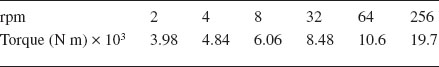
Calculate the shear stress, shear rate, and viscosity for this material, and fit a suitable viscosity model to this data set.
39. A kaolin-in-water suspension was tested in a 13 mm internal diameter horizontal tube, and the following data were reported:
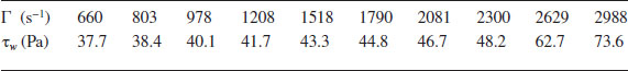
Obtain the true shear stress, shear rate, and viscosity for this suspension. Does this suspension exhibit a yield stress? Fit a suitable viscosity model to approximate the rheology of this suspension.
40. The same suspension as that in Problem 39 above was subsequently tested in a 28 mm internal diameter pipe, and the following data reported:
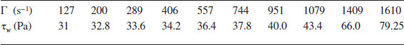
Obtain the true shear stress, shear rate, and viscosity for this material using this information. Is this consistent with the results obtained in Problem 39? If not, give possible reasons.
Ay |
Area whose outward normal vector is in the y direction, [L2] |
Fx |
Force component in the x direction, [F = M L/t2] |
fn() |
A function of whatever is in the () |
G |
Shear modulus, [F/L2 = M/Lt2] |
g |
Acceleration due to gravity, [L/t2] |
hy |
Distance between plates in the y direction, [L] |
L |
Length, [L] |
m |
Power law consistency parameter, [M/(Lt2-n)] |
n |
Power law flow index, [—] |
n′ |
Variable defined by Equation 3.14 or 3.18, [—] |
P |
Pressure, [F/L2 = M/Lt2] |
p |
Parameter in Carreau model, [—] |
Q |
Volumetric flow rate, [L3/t] |
R |
Radius, [L] |
r |
Radial direction or coordinate, [L] |
SG |
Specific gravity, [—] |
T |
Temperature (absolute), [T] |
T |
Torque or moment, [FL = M L2/t2] |
Ux |
Displacement of boundary in the x direction, [L] |
ux |
Local displacement in the x direction, [L] |
vx |
Local velocity component in x direction, [L/t] |
V |
Bulk or average velocity, [L/t] |
z |
Vertical direction measured upward, [L] |
GREEK
β |
(Ri/Ro) ratio of inner to outer radius in Couette viscometer |
Γ |
Shear rate at tube wall for Newtonian fluid, Equation 3.16, [1/t] |
γyx |
Gradient of x displacement in y direction (shear strain, or γ), [—] |
Gradient of x velocity in y direction (shear rate, or ), [1/t] |
|
Δ() |
Value of ()2 − ()1 |
λ |
Fluid time constant parameter, [t] |
μ |
Viscosity (Newtonian), [M/Lt] |
μ∞ |
Bingham limiting viscosity, [M/Lt] |
η |
Viscosity function (non-Newtonian), [M/Lt] |
ρ |
Density, [M/L3] |
θ |
Angular displacement, [—] |
τo |
Yield stress, [F/L2 = M/Lt2] |
τyx |
Force in x direction on y surface (shear stress, or τ), [F/L2 = M/Lt2] |
τrθ |
Force in θ direction on r surface (shear stress), [F/L2 = M/Lt2] |
Φ |
Static potential = P+ρgz, [F/L2 = M/L t2] |
Ω |
Angular velocity of boundary, [1/t] |
SUBSCRIPTS
1 |
Reference point 1 |
2 |
Reference point 2 |
i |
Inner |
o |
Outer |
o |
Zero shear rate parameter |
w |
Value at wall |
x, y, r, θ |
Coordinate directions |
∞ |
High shear limiting parameter |
Barnes, H.A., J.F. Hutton, and K. Walters, An Introduction to Rheology, Elsevier, New York, 1989.
Boger, D.V. and K. Walters, Rheological Phenomena in Focus, Elsevier, Amsterdam, the Netherlands, 1992.
Carreau, P.J., Rheological equations from molecular network theories, Trans. Soc. Rheol., 16, 99–127, 1972.
Chhabra, R.P. and J.F. Richardson, Non-Newtonian Flow and Applied Rheology, 2nd edn., Butterworth-Heinemann, Oxford, U.K., 2008.
Darby, R., Viscoelastic Fluids, Marcel Dekker, New York, 1976.
Darby, R., Couette viscometer data reduction for materials with a yield stress, J. Rheology, 29, 369–378, 1985.
Darby, R. and S. Pivsa-Art, An improved correlation for turbulent drag reduction in dilute polymer solutions, Can. J. Chem. Eng., 69, 1395–1400, 1991.
Meter, D.M., Tube flow of non-Newtonian polymer solutions: Part I, Laminar flow and rheological models, AIChE J., 10, 878–881, 1964.
Probstein, R.F., Physico-Chemical Hydrodynamics: An Introduction, Wiley, New York, 2003.
Reid, R.C., J.M. Prausnitz, and T.K. Sherwood, The Properties of Gases and Liquids, 3rd edn., McGraw-Hill, New York, 1977.
Yasuda, K., R.C. Armstrong, and R.E. Cohen, Shear flow properties of concentrated solutions of linear and star branched polystyrenes, Rheol. Acta, 20, 163–178, 1981.
Yaws, C.L., X. Lin, and L. Bu, Calculate viscosities for 355 liquids, Chem. Eng., 101, 119–126, April 1994.
* “Rheology” is the study of the deformation and flow behavior of materials, both fluids and solids. See for example: Darby (1976), Barnes et al. (1989), Boger and Walters (1992), etc.
* Conversion Factors for viscosity include: 1 poise = 1 dyn s/cm2 = 100 cP = 0.1 N s/m2 0.1 Pa s = 1 gm/(cm s) = 0.0672 lbm/(ft s) = 2.09 × 10⁻³ lbf s/ft2.