7	Internal Flow Applications

“Take the best that exists and make it better. If it does not exist, design it.”

—Henry Royce, 1863–1933, Engineer

I.    NONCIRCULAR CONDUITS

All the relationships presented in Chapter 6 apply directly to circular pipes. However, many of these results caSn also, with appropriate modifications, be applied to conduits with noncircular cross sections. It should be recalled that the derivation of the momentum equation for uniform flow in a tube, for example, Equation 5.44, involved no assumption about the shape of the tube cross section. The result is that the friction loss is a function of a geometric parameter called the “hydraulic diameter”:

$D_h=4\frac{A}{W_p}$

(7.1)

where

A is the area of the flow cross section

W_p is the wetted perimeter (i.e., the length of contact between the fluid and the solid boundary in the flow cross section)

For a full circular pipe, D_h = D (the pipe diameter). The hydraulic diameter is the key characteristic geometric parameter for a conduit with any cross-sectional shape.

A.    LAMINAR FLOWS

By either integrating the microscopic momentum equations (see Example 5.9) or applying a momentum balance to a “slug” of fluid in the center of the conduit as was done for tube flow, a relationship can be determined between flow rate and driving force for laminar flow in a conduit with a noncircular cross section. This can also be done by the application of the equivalent integral expressions analogous to Equations 6.6 through 6.10. The results for a few examples for Newtonian fluids will be given in the following. These results are the equivalent of the Hagen–Poiseuille equation for a circular tube and are given in both dimensional and dimensionless form.

1.  Flow in a Slit

Flow between two flat parallel plates that are closely spaced (h ≪ W) is shown in Figure 7.1.

The hydraulic diameter for this geometry is D_h = 4A/W_p = 4hW/2W = 2h, and the solution for a Newtonian fluid in laminar flow (analogous to Equation 6.11 for tube flow) is

$Q=-\frac{\Delta \Phi W{h}^3}{12\text{μ}L}$

(7.2)

This can be rearranged into the equivalent dimensionless form

$f{N}_{Re,h}=24$

(7.3)

FIGURE 7.1 Flow in a slit.

where

$N_{Re,h}=\frac{D_{h}V\text{ρ}}{\text{μ}}=\frac{D_{h}Q\text{ρ}}{\text{μ}A}$

(7.4)

Here, A = Wh, and the Fanning friction factor is, by definition,

$f=\frac{e_f}{\left(V^2\text{/}2\right)\left(4L\text{/}{D}_h\right)}=\frac{-\Delta \Phi }{\left(\text{ρ}{V}^2\text{/}2\right)\left(4L\text{/}{D}_h\right)}$

(7.5)

and the Bernoulli equation reduces to e_f = −ΔΦ/ρ for this system.

2.  Flow in a Film

The flow of a thin film down an inclined plane is illustrated in Figure 7.2. The film thickness is h ≪ W, and the plate is inclined at an angle θ to the vertical. For this flow, the hydraulic diameter is D_h = 4hW/W = 4h (since only one boundary in the cross section is a wetted surface). The laminar flow solution for a Newtonian fluid is

$Q=-\frac{\Delta \Phi h^{3}W}{3\text{μ}L}=\frac{\text{ρ}g{h}^{3}W\cos \text{θ}}{3\text{μ}}$

(7.6)

The dimensionless form of this equation is

$f{N}_{Re,h}=24$

(7.7)

where the Reynolds number and friction factor are given by Equations 7.4 and 7.5, respectively.

FIGURE 7.2 Flow in a film.

3.  Annular Flow

Axial flow in the annulus between two concentric cylinders, as illustrated in Figure 7.3, is frequently encountered in tubular heat exchangers and coating devices. For this geometry, the hydraulic diameter is $D_h=4\left(\text{π/}4\right)\left(D_o^2-D_i^2\right)/\left[\text{π}\left(D_o+D_i\right)\right]=D_o-D_i$, and the Newtonian laminar flow solution is

$Q=-\frac{\text{ΔΦπ}\left(D_o^2-D_i^2\right)}{128\text{μ}L}\left(D_o^2+D_i^2-\frac{D_o^2-D_i^2}{\ln \left(D_o/D_i\right)}\right)$

(7.8)

The dimensionless form of this expression is

$f{N}_{Re,h}=16\text{α}$

(7.9)

where

$\text{α}=\frac{{\left(D_o-D_i\right)}^2}{D_o^2+D_i^2-\left(D_o^2-D_i^2\right)/\ln \left(D_o/D_i\right)}$

(7.10)

It can be shown that as D_i/D_o → 0, α → 1 and the flow approaches that for a circular tube. Likewise, as D_i/D_o → 1, α → 1.5 and the flow approaches that for a slit.

It is seen that the value of fN_{Re, h} for laminar flow in a wide variety of geometries varies only by about a factor of 50% or so. This value has been determined for a Newtonian fluid in various geometries, and the results are summarized in Table 7.1. This table gives the expressions for the crosssectional area and hydraulic diameter for six different conduit geometries and the corresponding values of fN_{Re, h}, the dimensionless laminar flow solution. The total range of values for fN_{Re, h} for all of these geometries is seen to be approximately 12–24. Thus, for any completely arbitrary geometry, the dimensionless expression fN_{Re, h} ≈ 18 would provide an approximate solution for fully developed laminar flow, with an error of about 30% or less.

B.    TURBULENT FLOWS

The effect of geometry on the flow field for turbulent flows is much less pronounced than for laminar flows. This is because the majority of the energy dissipation or flow resistance occurs within the boundary layer which, in typical turbulent flows, occupies a relatively narrow region of the total flow field near the boundary. This is in contrast to laminar flows, where the “boundary layer” occupies the entire flow field. Thus, although the total solid surface contacted by the fluid in turbulent flows influences the flow resistance, the actual shape of the boundary surface is not as important. Consequently, the hydraulic diameter provides an even better characterization of the effect of geometry for noncircular conduits with turbulent flows than with laminar flows. The result is that relationships developed for turbulent flows in circular pipes can be applied directly to conduits of noncircular cross section simply by replacing the tube diameter by the hydraulic diameter in the relevant dimensionless groups. The accuracy of this procedure increases with increasing Reynolds number because the higher the Reynolds number, the greater the turbulence intensity, and the thinner the boundary layer, hence the less important the actual shape of the cross section.

FIGURE 7.3 Flow in an annulus.

TABLE 7.1

Laminar Flow Factors for Noncircular Conduits

It is important to use the hydraulic diameter substitution (D = D_h) in the appropriate (original) form of the dimensionless groups (e.g., N_Re = DVρ/μ, f = e_f/(2LV²/D), ε/D) and not a form that has been adapted for circular tubes (e.g., N_Re = 4Qρ/πDμ). That is, the proper modification of the Reynolds number for a noncircular conduit is (D_hVρ/μ), not (4Qρ/πD_hμ). One clue that the dimensionless group is of the wrong form for a noncircular conduit is the presence of π, which is normally associated only with circular geometries (remember, “pi are round, cornbread are square”). Thus, the appropriate dimensionless groups from the tube flow solutions can be modified for noncircular geometries as follows:

$N_{Re,h}=\frac{D_{h}V\text{ρ}}{\text{μ}}=\frac{4Q\text{ρ}}{W_p\text{μ}}$

(7.11)

$f=\frac{e_f{D}_h}{2L{V}^2}=\frac{2e_f}{L{Q}^2}\left(\frac{A^3}{W_p}\right)$

(7.12)

$N_R=\frac{N_{Re,h}}{\text{ε/}{D}_h}=\frac{D_h^{2}Q\text{ρ}}{\text{ε}A\text{μ}}=\frac{16Q\text{ρ}}{\text{εμ}}=\frac{16Q\text{ρ}}{\text{εμ}}\left(\frac{A}{W_p^2}\right)$

(7.13)

$f{N}_{Re,h}^2=\frac{32e_f{\text{ρ}}^2}{L{\text{μ}}^2}{\left(\frac{A}{W_p}\right)}^3=\frac{e_f{\text{ρ}}^2{D}_h^3}{2L{\text{μ}}^2}$

(7.14)

$f{N}_{Re,h}^5=\frac{2048e_f{Q}^3{\text{ρ}}^5}{L{\text{μ}}^5}{\left(\frac{A}{W_p^2}\right)}^3$

(7.15)

The circular tube expressions for f and N_Re containing π can also be transformed to the equivalent expressions for a noncircular conduit by the substitution

$\text{π}\to \frac{W_p}{D_h}=4\frac{A}{D_h^2}=\frac{1}{4}\frac{W_p^2}{A}$

(7.16)

II.    MOST ECONOMICAL DIAMETER

In the previous chapter, we saw how to determine the driving force (e.g., pumping requirement) required to deliver a specified flow rate through a given pipe size, as well as how to determine the proper pipe size that will deliver a specified flow rate for a given driving force (e.g., pump head). However, when we install a pipeline or piping system, we are normally free to select both the “best” pipe and the “best” pump. The term “best” in this case refers to that combination of pipe and pump that will minimize the total system cost.

The total system cost of a pipeline or piping system includes the fixed capital cost of both the pipe (including valves and fittings) and pumps, as well as the continuous operating costs, that is, the cost of the energy required to drive the pumps, maintenance cost, etc.:

Capital cost of pipe (CCP)

Capital cost of pump stations (CCPS)

Energy cost to power pumps (EC)

Although the energy cost is “continuous” and the capital costs are “one time,” it is common to spread out (or amortize) the capital cost over a period of Y years, that is, over the “economic lifetime” of the pipeline. The reciprocal of this (X = 1/Y) is the fraction of the total capital cost written off per year. Thus, taking 1 year as the time basis, we can combine the capital cost per year and the energy cost per year to get the total annual cost. We may also factor in a cost for maintenance, which will be a fraction M of the total cost of pipe and pump stations. This is typically about 2% of total installed cost.

Data on the cost of typical pipeline installations of various sizes (including valves and fittings) were reported by Darby and Melson (1982). They showed that these data can be represented by the equation

$CCP=a{D}_{ft}^{p}L$

(7.17)

where

D_ft is the pipe ID in feet

the parameters a and p depend upon the pipe wall thickness as shown in Table 7.2

Likewise, the capital cost of (installed) pump stations (for 500 hp and over) was shown to be a linear function of the pump power (see Figure 7.4):

$CCPS=\left(A+B\frac{HP}{{\text{η}}_e}\right)\left(1+M\right)$

(7.18)

where

A = $172,800

B = $451 hp⁻¹ (in 1980 dollars)

HP/η_e is the horsepower rating of the pump (HP is the “hydraulic power,” which is the power delivered directly to the fluid and η_e is the pump efficiency)

M accounts for maintenance costs, which are typically about 2%/year

The energy cost is determined from the power required to drive the pumps, which is the product of the mass flow rate and the pump work per unit mass of fluid, as determined from the Bernoulli equation:

$-w=\frac{\text{ΔΦ}}{\text{ρ}}+\frac{1}{2}\text{Δ}{V}^2+{\displaystyle \sum e_f}$

(7.19)

Table 7.2

Cost of Pipe (in 1980 Dollars)^a

Note:  The ANSI pipe grades correspond approximately to Sch. 20, 30, 40, 80, and 120 for commercial steel pipe.

^a  Pipe cost ($/ft) =a (ID_ft)^p.

FIGURE 7.4 Cost of pump stations (in 1980 dollars). Pump station cost ($) = CCPS = A + B hp/η_e where A = 172,800 and B = 451/hp for stations of 500 hp or more.

where

${\displaystyle \sum e_f}=4f\frac{V^2}{2}{\displaystyle \sum {\left(\frac{L}{D}\right)}_{eq}}$

(7.20)

and Σ(L/D)_eq is assumed to include the equivalent length of any fittings (which are usually a small portion of a long pipeline) as well as a maintenance factor. The required hydraulic pumping power (HP) is thus

$HP=-w\dot{m}=\dot{m}\left[\frac{2f{L}_{eq}{V}^2}{D}+\frac{\Delta \Phi }{\text{ρ}}\right]=\frac{32f{L}_{eq}{\dot{m}}^3}{{\text{π}}^2{\text{ρ}}^2{D}^5}+\dot{m}\frac{\Delta \Phi }{\text{ρ}}$

(7.21)

The total pumping energy cost per year is therefore

$EC=C\frac{HP}{{\text{η}}_e}$

(7.22)

where

C is the unit energy cost (e.g., $/(hp year), ȼ/kWh)

η_e is the pump efficiency

Note that the capital cost increases almost linearly with the pipe diameter, whereas the energy cost decreases in proportion to about the fifth power of the diameter.

The total annual cost of the pipeline is the sum of the capital and energy costs:

$TC=X\left(1+M\right)\left(CCP+CCPS\right)+EC$

(7.23)

Substituting Equations 7.17, 7.18, and 7.22 into Equation 7.23 gives

$TC=X\left(1+M\right)\left(a{D}^{p}L+A\right)+\frac{BX\left(1+M\right)+C}{{\text{η}}_e}\left[\frac{32fL{\dot{m}}^3}{{\text{π}}^2{\text{ρ}}^2{D}^5}+\dot{m}\frac{\Delta \Phi }{\text{ρ}}\right]$

(7.24)

Now, we wish to find the pipe diameter that minimizes this total cost. To do this, we differentiate Equation 7.24 with respect to D, set the derivative equal to zero, and solve for D (i.e., D_ec, the most economical diameter). The resulting expression for D_ec is

$D_{ec}={\left[\frac{B\left(1+M\right)+CY}{ap{\text{η}}_e\left(1+M\right)}\left(\frac{160f{\dot{m}}^3}{{\text{π}}^2{\text{ρ}}^2}\right)\right]}^{1/\left(p+5\right)}$

(7.25)

where Y = 1/X is the “economic lifetime” of the pipeline.

One might question whether the cost information in Table 7.2 and Figure 7.4 could be used today because these data are based on 1980 information and prices have increased greatly since that time. However, as seen from Equation 7.25, the cost parameters (i.e., B, C, and a) appear as a ratio. Because capital costs and energy costs tend to inflate at approximately the same rate (see, e.g., Durand et al., 1999), this ratio is essentially independent of inflation, and conclusions based on 1980 economic data should be valid today. However, this assumes that both capital costs (i.e., B and a) and energy costs (C) are based on the same year. If present-day energy costs are used, an inflation rate can be applied to the capital costs (B and a) to adjust them to present-day values by multiplying B and a by the factor (1 + i)^(t−1980) (e.g., Penoncello, 2015), where i is the average inflation rate (in decimal form) from 1980 to the present year t.

A.    NEWTONIAN FLUIDS

Equation 7.25 is implicit in the economic diameter, D_ec, because the friction factor (f) depends upon D_ec through the Reynolds number and the relative roughness of the pipe. It can be solved by iteration in a straightforward manner, however, by applying the procedure used for the “unknown diameter” problem in Chapter 6. That is, first assume a value for f (say, 0.005), calculate D_ec from Equation 7.25, and use this diameter to compute the Reynolds number and relative roughness. Then use these values to find f (from the Moody diagram or Churchill equation). If this value differs from the originally assumed value, use it in place of the assumed value and repeat the process until successive values of f agree.

Another approach is to regroup the characteristic dimensionless variables in the problem so that the unknown (D_ec) appears in only one group. After rearranging Equation 7.25 for f, we see that the following group will be independent of D_ec:

$f{N}_{Re}^{p+5}={\left(\frac{4}{\text{π}}\right)}^{p+3}\frac{{\text{ρ}}^2\left(1+M\right)ap{\text{η}}_e{\dot{m}}^{p+2}}{10\left[B\left(1+M\right)+CY\right]{\text{μ}}^{p+5}}=N_c$

(7.26)

We can call this the “cost group” (N_c) because it contains all of the cost parameters (a, B and C). We can also define a roughness group that does not include the diameter:

$N_R=\frac{\text{ε/}{D}_{ec}}{N_{Re}}=\frac{\text{πμε}}{4\dot{m}}$

(7.27)

The remaining group is the Reynolds number, which is the dependent group because it alone contains D_ec:

$N_{Re}=\frac{4\dot{m}}{\text{π}{D}_{ec}\text{μ}}$

(7.28)

The Moody diagram can be used to construct a plot of N_Re versus $N_c=f{N}_{Re}^{p+5}$ for various values of p and N_R (a double-parametric plot), which permits a direct solution to this problem (see Darby and Melson, 1982). These equations can also be used directly to simplify the iterative solution. Since the value of N_c is known, assuming a value for f will give N_Re directly from Equation 7.26. This, in turn, gives D_ec from Equation 7.28 and hence ε/D_ec. These values of N_Re and ε/D_ec are used to find f from the Moody diagram or Churchill equation, and the iteration is continued until successive values of f agree. The most difficult aspect of working with these groups is ensuring a consistent set of units for all the variables (with appropriate use of the conversion factor g_c, if working in engineering units). For this reason, it is easier to work with consistent units in a scientific system (e.g., SI or cgs), which avoids the need for g_c.

B.    NON-NEWTONIAN FLUIDS

A procedure analogous to the one followed above for Newtonian fluids can be used for non-Newtonian fluids that follow the power law or Bingham plastic models (Darby and Melson, 1982), as follows:

1.  Power Law Fluid

For power law fluids, the basic dimensionless variables are the Reynolds number, the friction factor, and the flow index (n). If the Reynolds number is expressed in terms of the mass flow rate, then

$N_{Re,pl}={\left(\frac{4}{\text{π}}\right)}^{2-n}{\left(\frac{4n}{3n+1}\right)}^n\left(\frac{{\dot{m}}^{2-n}{\text{ρ}}^{n-1}}{D_{ec}^{4-3n}{8}^{n-1}m}\right)$

(7.29)

Eliminating D_ec from Equations 7.25 and 7.29, the equivalent cost group becomes

$f^{4-3n}{N}_{Re,pl}^{5+p}=\frac{\left(52.4\right)\left({10}^{3n}\right)\left(2^{7p-3n\left(1+p\right)}\right)}{p^{\left(2+n\right)\left(1+p\right)}{m}^{5+p}}{\left(\frac{ap{\text{η}}_e}{B+CY}\right)}^{4-3n}\left(\frac{{\text{ρ}}^{3-p+n\left(p-1\right)}{\dot{m}}^{2\left(p-1\right)+n\left(4-p\right)}}{{\left[\left(3n+1\right)/n\right]}^{n\left(5+p\right)}}\right)$

(7.30)

Since all values on the right-hand side of Equation 7.30 are known, assuming a value of f allows a corresponding value of N_{Re, pl} to be determined. This value can then be used to check the assumed value of f using the general expression for the power law friction factor (Equation 6.44 for laminar flow or Equation 6.46 for turbulent flow) and iterating until agreement is attained. (Note: The maintenance cost factor has not been included in these equations, but it can easily be accounted for by multiplying the terms a and B by the factor [1 + M]).

2.  Bingham Plastic

The basic dimensionless variables for the Bingham plastic are the Reynolds number, the Hedstrom number, and the friction factor. Eliminating D_ec from the Reynolds number and Equation 7.25 (as mentioned earlier), the cost group is

$f{N}_{Re}^{p+5}={\left(\frac{4}{\text{π}}\right)}^{p+3}\frac{{\text{ρ}}^{2}ap{\text{η}}_e{\dot{m}}^{p+2}}{10\left(B+CY\right){\text{μ}}_{\infty \yen }^{p+5}}$

(7.31)

D_ec can also be eliminated from the Hedstrom number by combining it with the Reynolds number:

$N_{He}{N}_{Re}^2={\left(\frac{4}{\text{π}}\right)}^2\frac{{\text{τ}}_o\text{ρ}{\dot{m}}^2}{{\text{μ}}_{\infty }^4}$

(7.32)

These equations can readily be solved by iteration, as follows. Assuming a value of f allows N_Re to be determined from Equation 7.31. This is then used with Equation 7.32 to find N_He. The friction factor is then calculated using these values of N_Re and N_He and the Bingham plastic pipe friction factor equation (Equation 6.65). The result is compared with the assumed value, and the process is repeated until agreement is attained.

Graphs have been presented by Darby and Melson (1982) that can be used to solve these problems directly without iteration. However, interpolation on double-parametric logarithmic scales is required, so only approximate results can be expected from the precision of reading these plots. As mentioned before, the greatest difficulty in using these equations is that of ensuring consistent units. In many cases, it is most convenient to use cgs units in problems such as these, because fluid properties (density and viscosity) are frequently found in these units and the scientific system (e.g., cgs) does not require the conversion factor g_c. In addition, the energy cost is frequently given in cents per kilowatt-hour, which is readily converted to cgs units (e.g., $/erg).

III.    FRICTION LOSS IN VALVES AND FITTINGS

Evaluation of the friction loss in valves and fittings involves the determination of the appropriate loss coefficient (K_f), which in turn defines the energy loss per unit mass of fluid:

$e_f=\frac{K_f{V}^2}{2}$

(7.33)

where V is (usually) the velocity in the pipe upstream of the fitting or valve. However, this is not always true and care must be taken to ensure that the value of V that is used is the one that is specified in the defining equation for K_f. The actual evaluation of K_f is done by determining the friction loss e_f from measurements of the pressure drop across the fitting (elbows, tees, valves, etc.). This is not straightforward, however, because the pressure in the pipe is influenced by the presence of the fitting for a considerable distance both upstream and downstream of the fitting. It is not possible, therefore, to obtain accurate values from measurements taken at pressure taps immediately adjacent to the fitting. The most reliable method is to measure the total pressure drop through a long run of pipe both with and without the fitting, at the same flow rate, and determine the fitting loss by difference.

There are several “correlation” expressions for K_f, which are described below (in Sections A through E) in the order of increasing accuracy. The “3-K” method (see Section E) is recommended because it accounts directly for the effect of both Reynolds number and fitting size on the loss coefficient and more accurately reflects the effect of fitting diameter than the 2-K method (Section D). For highly turbulent flow, the Crane method (Section C) agrees well with the 3-K method but is less accurate at low Reynolds numbers and is not recommended for laminar flow. The loss coefficient and (L/D)_eq methods are more approximate but give acceptable results at high Reynolds (fully turbulent flow) numbers and when losses in valves and fittings are “minor losses” compared to the pipe friction. They are also appropriate for first estimates in problems that require iterative solutions.

A.    LOSS COEFFICIENT

Values of K_f for various types of valves, fittings, etc., are found tabulated in various textbooks and handbooks. The assumption that these values are constant for a given type of valve or fitting is not accurate, however, because in reality the value of K_f varies with both the size (scale) of the fitting and the level of turbulence (Reynolds number). One reason that K_f is not the same for all fittings of the same type (e.g., all 90° elbows) is that all the dimensions of a fitting, such as the diameter and radius of curvature, do not scale by the same factor for large and small fittings. Most tabulated values for constant K_f values are close to the values of K_∞ from the 3-K method.

B.    EQUIVALENT L/D METHOD

The basis for the (L/D)_eq method is the assumption that there is some length of pipe (L_eq) that has the same friction loss as that which occurs in the fitting, at a given (pipe) Reynolds number. Thus, the fittings are conceptually replaced by the equivalent additional length of pipe that has the same friction loss as the fitting:

$e_f=\frac{4f{V}^2}{2}{\displaystyle \sum {\left(\frac{L}{D}\right)}_{eq}}$

(7.34)

where f is the Fanning friction factor in the pipe at the given pipe Reynolds number and relative roughness. This is a convenient concept because it allows the solution of pipe flow problems with fittings to be carried out in a manner identical to that without fittings if L_eq is known. Values of (L/D)_eq are tabulated in various textbooks and handbooks for a variety of fittings and valves (and are also listed in Table 7.3 here). The method assumes that (1) sizes of all fittings of a given type can be scaled by the corresponding pipe diameter (D), and (2) the influence of turbulence level (i.e., Reynolds number) on the friction loss in the fitting is identical to that in the pipe (because the pipe f value is used to determine the fitting loss). Neither of these assumptions is accurate (as pointed out earlier), although the approximation provided by this method gives reasonable results at high turbulence levels (fully turbulent flow), especially if fitting losses are minor when compared to the total pipe friction loss.

Table 7.3

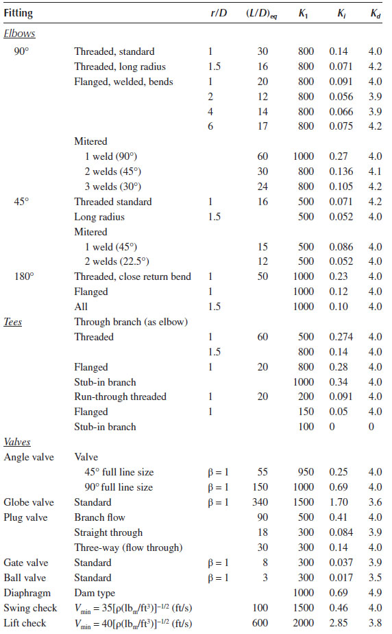
3-K Constants^a for Loss Coefficients for Valves and Fittings

Note:  D_n is the nominal pipe size in inches.

^a  $K_f=\frac{K_1}{N_{Re}}+K_i\left(1+\frac{K_d}{D_n^{0.3}}\right).$

C.    CRANE METHOD

The method given in the Crane Technical Paper 410 (1991) is a modification of the aforementioned methods. It is equivalent to the (L/D)_eq method except that it recognizes that there is generally a higher degree of turbulence in the fitting than in the pipe at a given (pipe) Reynolds number. This is accounted for by always using the “fully turbulent” value for f (e.g., f_T) in the expression for the friction loss in the fitting, regardless of the actual Reynolds number in the pipe, that is,

$e_f=\frac{K_f{V}^2}{2}\text{where}{K}_f=4f_T\left(\frac{L}{D}\right){}_{eq}$

(7.35)

The value of f_T can be calculated from the Colebrook equation (Equation 6.40), for example,

$f_T=\frac{0.0625}{{\left[\log \left(3.7D\text{/ε}\right)\right]}^2}$

(7.36)

in which ε is the pipe roughness (0.0018 in. for new commercial steel). This is a two-constant model [f_T and (L/D)_eq], and values of these constants are tabulated in the Crane paper for a wide variety of fittings, valves, etc. This method gives satisfactory results for high turbulence levels (fully turbulent flow) but is less accurate at low Reynolds numbers and does not scale well with pipe size.

D.    2-K (HOOPER) METHOD

The 2-K method by Hooper (1981, 1988) was based on experimental data from a variety of valves and fittings over a wide range of Reynolds numbers. The effect of both the Reynolds number and scale (fitting size) is reflected in the expression for the loss coefficient:

$e_f=\frac{K_f{V}^2}{2},\text{where}{K}_f=\frac{K_1}{N_{Re}}+K_{\infty }\left(1+\frac{1}{I{D}_{in.}}\right)$

(7.37)

Here, ID_in. is the internal diameter (in inches) of the pipe that contains the fitting. This method is valid over a much wider range of Reynolds numbers than the other methods. However, the effect of pipe size (e.g., 1/ID_in.) in Equation 7.37 does not accurately reflect the scaling with pipe size, as discussed below in Section E.

E.    3-K (DARBY) METHOD

Although the 2-K method applies over a wide range of Reynolds numbers, the scaling term (1/ID) does not accurately reflect data over a wide range of sizes for valves and fittings, as reported in a variety of sources (Crane, 1991; CCPS, 1998; Perry and Green, 2007; Darby, 2001; and references cited therein). Specifically, all the preceding methods tend to underpredict the friction loss for fittings of larger diameters. Darby (2001) has evaluated data from the literature for various valves and fittings and found that they can be represented more accurately by the following “3-K” equation:

$K_f=\frac{K_1}{N_{Re}}+K_i\left(1+\frac{K_d}{D_{n,in.}^{0.3}}\right)$

(7.38)

Note that D_n,in. is the nominal diameter, in inches. The values of the 3 K’s (K₁, K_i, and K_d) are given in Table 7.3 (along with representative values of (L/D)_eq) for various valves and fittings. These values were determined from combinations of literature values from the references listed earlier and were all found to accurately follow the scaling law given in Equation 7.38. The values of K₁ are mostly those of the Hooper 2-K method, and the values of K_i were mostly determined from the Crane data. However, since there is no single comprehensive data set for many fittings over a wide range of sizes and Reynolds numbers, some estimation was necessary for some values.

Values of K_d are all very close to 4.0, and this value can be used to scale known values of K_f for a given pipe size to apply to other sizes. This method is the most accurate of the methods described for all Reynolds numbers and fitting sizes. Tables 7.4 and 7.5 list values for K_f for expansions and contractions and entrance and exit conditions, respectively (Hooper, 1981). The definition of K_f (i.e., K_f = 2e_f/V²) involves the kinetic energy of the fluid, V²/2. For sections that undergo area changes (e.g., pipe entrance, exit, expansions, or contractions), the entering and leaving velocities will be different. Because the value of the velocity used with the definition of K_f is arbitrary, it is very important to know which velocity is the reference value for a given loss coefficient. Values of K_f are usually based on the larger velocity entering or leaving the fitting (through the smaller cross section), but this should be verified if any doubt exists.

A note is in order regarding the exit loss coefficient, which is listed in Table 7.5 as equal to 1.0. Actually, if the fluid exits the pipe in a free jet into unconfined space, the loss coefficient is zero because the velocity of the fluid exiting the pipe is close to that of the fluid inside the pipe and thus the kinetic energy change is zero. However, when the fluid exits into a confined space so that the fluid leaving the pipe immediately mixes with the same fluid in the receiving vessel, the kinetic energy is dissipated as friction loss in the mixing process so the velocity goes to zero, and thus the loss coefficient is 1.0. In this case, the change in the kinetic energy and the friction loss at the exit cancel out.

IV.    NON-NEWTONIAN FLUIDS

There are insufficient data in the literature to enable reliable correlation or prediction of friction loss in valves and fittings for non-Newtonian fluids. As a first approximation, however, it can be assumed that a correlation similar to the 3-K method should apply to non-Newtonian fluids if the (Newtonian) Reynolds number in Equation 7.38 could be replaced by a single corresponding dimensionless group that adequately incorporates the influence of the non-Newtonian properties. For the power law and Bingham plastic fluid models, two rheological parameters are required to describe the viscous properties, which generally results in two corresponding dimensionless groups (N_Re,pl and n for the power law and N_Re and N_He for the Bingham plastic). However, it is possible to define an “effective viscosity” for a non-Newtonian fluid model that has the same significance in the Reynolds number as the viscosity has for a Newtonian fluid and incorporates all of the appropriate parameters for that model, which then can be used to define an equivalent non-Newtonian Reynolds number (see Darby and Forsyth, 1992). For a Newtonian fluid, the Reynolds number can be rearranged as follows:

$N_{Re}=\frac{DV\text{ρ}}{\text{μ}}=\frac{\text{ρ}{V}^2}{\text{μ}V\text{/}D}=\frac{\text{ρ}{V}^2}{{\text{τ}}_w\text{/}8}$

(7.39)

Table 7.4

Loss Coefficients for Expansions and Contractions

Kf to be used with upstream velocity head, $V_1^2/2$. β =d/D

Contraction

θ < 45°

NRe,1 < 2500:

$K_f=1.6\left[1.2+\frac{160}{N_{\mathrm{Re},1}}\right]\left[\frac{1}{{\beta }^4}-1\right]\sin \frac{\theta }{2}$

NRe,1 > 2500:

$K_f=1.6\left[0.6+1.92f_1\right]\left[\frac{1-{\beta }^2}{{\beta }^4}\right]\sin \frac{\theta }{2}$

θ > 45°

NRe,1 < 2500:

$K_f=\left[1.2+\frac{160}{N_{\mathrm{Re},1}}\right]\left[\frac{1}{{\beta }^4}-1\right]{\left[\sin \frac{\theta }{2}\right]}^{1/2}$

NRe,1 > 2500:

$K_f=\left[0.6+1.92f_1\right]\left[\frac{1-{\beta }^2}{{\beta }^4}\right]{\left[\sin \frac{\theta }{2}\right]}^{1/2}$

Expansion

θ < 45°

NRe,1 < 4000:

$K_f=5.2\left(1-{\beta }^4\right)\sin \frac{\theta }{2}$

NRe,1 > 4000:

$K_f=2.6\left(1+3.2f_1\right){\left(1-{\beta }^2\right)}^2\sin \frac{\theta }{2}$

θ > 45°

NRe,1 < 4000:

$K_f=2\left(1-{\beta }^4\right)$

NRe,1 > 4000:

$K_f=\left(1+3.2f_1\right){\left(1-{\beta }^2\right)}^2$

Source:  Hooper, W.B., “Calculate head Loss Caused by Change in Pipe Size”, Chem. Eng., 95, pp. 89–92, 1988.

Note:  N_Re,1 is the upstream Reynolds number, and f₁ is the pipe friction factor at this Reynolds number.

Table 7.5

Loss Coefficients for Pipe Entrance and Exit

Source:  Hooper, W.B., “The 2-K Method Predicts Head Loss in Pipe Fittings” Chem. Eng., 88, pp. 96–100, 1981.

Introducing τ_w = m[(8V/D)(3n + 1)/4n]ⁿ for the power law model results in

$N_{Re,pl}=\frac{2^{\left(7-3n\right)}\text{ρ}{Q}^{\left(2-n\right)}}{m{\text{π}}^{\left(2-n\right)}{D}^{\left(4-3n\right)}}{\left(\frac{n}{3n+1}\right)}^n$

(7.40)

which is identical to the expression derived in Chapter 6 (see Equation 6.71).

For the Bingham plastic, replacing τ_w for the Newtonian fluid in Equation 7.39 with ${\text{τ}}_o+{\text{μ}}_{\infty }{\dot{\gamma }}_w$ and using the approximation ${\dot{\gamma }}_w=8V\text{/}D$, the corresponding expression for the Reynolds number is

$N_{Re,BP}=\frac{4Q\text{ρ}}{\text{π}D{\text{μ}}_{\infty }\left(1+\text{π}{D}^3{\text{τ}}_o/32Q{\text{μ}}_{\infty }\right)}=\frac{N_{Re}}{1+N_{He}\text{/}8N_{Re}}$

(7.41)

The ratio N_He/N_Re = Dτ_o/Vμ_∞ is also called the Bingham number (N_Bi). Darby and Forsyth (1992) showed experimentally that mass transfer in Newtonian and non-Newtonian fluids can be correlated by this method. That is, the same dimensionless correlation can be applied to both Newtonian and non-Newtonian fluids when the Newtonian Reynolds number is replaced by either Equation 7.40 for the power law fluid or Equation 7.41 for the Bingham plastic model. As a first approximation, therefore, we may assume that the same method would apply to friction loss in valves and fittings as described by the 3-K model, Equation 7.38. This approach is in agreement with the scant literature data on fitting losses with power law and Bingham plastic fluids (see, e.g., Chhabra and Richardson, 2008).

V.    PIPE FLOW PROBLEMS WITH FITTINGS

The inclusion of significant friction loss in fittings in piping systems requires a somewhat different procedure for the solution of flow problems than that which was used in the absence of fitting losses (see Chapter 6). We will consider the same classes of problems as before, that is, the unknown driving force, the unknown flow rate, and the unknown diameter problems for Newtonian, power law, and Bingham plastic fluids. The governing equation, as before, is the Bernoulli equation written in the form

$DF=-\left(\frac{\text{ΔΦ}}{\text{ρ}}+w\right)={\displaystyle \sum _{pipe+fittings}{e}_f+\frac{1}{2}\Delta \left(\text{α}{V}^2\right)}$

(7.42)

where

${\displaystyle \sum _{Pipe+Fittings}{e}_f=\frac{1}{2}}{\displaystyle \sum _{Pipe+Fittings}\left(V^2{K}_f\right)=\frac{8Q^2}{{\text{π}}^2}}{\displaystyle \sum _{Pipe+Fittings}\frac{K_f}{D^4}}$

(7.43)

$K_{pipe}=\frac{4fL}{D},K_{fittings}=\frac{K_1}{N_{Re}}+K_i\left(1+\frac{K_d}{D_n^{0.3}}\right)$

(7.44)

The summation is over each length of pipe and each fitting of diameter D in the system. The expressions for the loss coefficients for the pipe and fittings are given in Equation 7.44. Substituting Equation 7.43 into 7.42 gives the following form of the Bernoulli equation:

$DF=\frac{8Q^2}{{\text{π}}^2}\left({\displaystyle \sum _{fi}\frac{K_{fi}}{D_i^4}+\frac{{\text{α}}_2}{D_2^4}-\frac{{\text{α}}_1}{D_1^4}}\right)$

(7.45)

Recall that the α’s are the KE correction factors at the upstream and downstream positions and that α = 2 for laminar flow and α “approx” = 1 for turbulent flow in a circular pipe for a Newtonian fluid. The same should apply (approximately) for non-Newtonian fluids, especially in the turbulent region.

A.    UNKNOWN DRIVING FORCE

Here, we wish to calculate the net driving force (pressure head, hydraulic head, or pump work) required to transport a given fluid at a given rate through a given piping system, containing a specified array of valves and fittings.

1.  Newtonian Fluid

The knowns and unknowns for this case are as follows:

Given: Q, μ, ρ, D_i, L_i, ε_i, fittings Find: DF

The driving force is given by Equation 7.45, in which the Ks are related to the other variables by the Moody diagram or Churchill equation for each pipe segment, (K_pipe,i), and by the 3-K method, Equation 7.44, for each valve and fitting (K_fit) as a function of the Reynolds number:

$N_{Re,i}=\frac{4Q\text{ρ}}{\text{π}{D}_i\text{μ}}$

(7.46)

The solution procedure is as follows:

1.  Calculate N_Re,i from Equation 7.46 for each pipe segment, valve, and fitting (i).

2.  For each pipe segment of diameter D_i, get f_i from the Churchill equation or Moody diagram using N_{Re, i} and ε_i/D_i, and calculate K_pipe,i = 4(fL/D)_i.

3.  For each valve and fitting, calculate K_fi from N_Rei and D_i using the 3-K method.

4.  Calculate the driving force, DF, from Equation 7.45.

2.  Power Law Fluid

The knowns and unknowns for this case are as follows:

Given: Q, D_i, L_i, m, n,ρ, fittings Find: DF

The appropriate expressions that apply are the Bernoulli equation (Equation 7.45), the power law Reynolds number (Equation 7.40), the pipe friction factor as a function of N_{Re, pl} (Equation 6.44), and the 3-K equation for fitting losses (Equation 7.38), with the power law Reynolds number. The solution procedure is as follows:

1.  From the given values, calculate N_Re,pl (Equation 7.40).

2.  Using Equation 6.44, calculate f and the corresponding K_pipe, and using the 3-K method, calculate the K_f for each fitting, Equation (7.38).

3.  Calculate the driving force, DF, from the Bernoulli equation, Equation 7.45.

3.  Bingham Plastic

The procedure is identical to that explained above, except that Equation 7.41 is used for the Reynolds number and Equation 6.65 is used for the pipe friction factor.

B.    UNKNOWN FLOW RATE

The Bernoulli equation, Equation 7.45, can be rearranged to solve for the flow rate Q as follows:

$Q=\frac{\text{π}}{2\sqrt{2}}{\left[\frac{DF}{{\displaystyle {\sum }_i\left(K_i\text{/}{D}_i^4\right)+{\text{α}}_2\text{/}{D}_2^4-{\text{α}}_1\text{/}{D}_1^4}}\right]}^{1/2}$

(7.47)

The flow rate can be readily calculated if the loss coefficients can be determined. The procedure involves iteration, starting with estimated values for the loss coefficients. These are then inserted into Equation 7.47 to find Q, which is then used to calculate the Reynolds number(s). The result is used to calculate revised values of the ${K^{\prime }}_f\text{s}$, as follows:

1.  Newtonian Fluid

The knowns and unknowns are as follows:

Given: DF, D, L, ε, μ, ρ Find: Q

1.  A first estimate for the pipe friction factor and the ${K^{\prime }}_f\text{s}$ can be made by assuming that the flow is fully turbulent (and that α₁ = α₂ = 1). From the Colebrook equation

$f_1=\frac{0.0625}{{\left[\log \left(3.7D\text{/ε}\right)\right]}^2}$

(7.48)

and

$K_{fit}\cong K_i\left(1+\frac{K_d}{D_{n,in.}^{0.3}}\right)$

(7.49)

2.  Use these values to calculate Q from Equation 7.47 and then the Reynolds number from N_Re = 4Qρ/πDμ.

3.  This Reynolds number is then used to determine a revised pipe friction factor and loss coefficient (K_{f, pipe} = 4fL/D) from the Churchill equation or the Moody diagram and the K_fit values from the 3-K equation.

4.  The solution is the last value of Q calculated from step 2.

2.  Power Law Fluid

The knowns and unknowns are as follows:

Given: DF, D, L, m, n, ρ Find: Q

The procedure is essentially identical to that explained above for the Newtonian fluid, except that Equation 7.40 is used for the Reynolds number in step 2 and Equation 6.47 is used for the pipe friction factor in step 3.

3.  Bingham Plastic

The knowns and unknowns are as follows:

Given: DF, D, L, μ_∞, τ_o, ρ Find: Q

The procedure is again analogous to that for the Newtonian fluid, except that the pipe friction factor in step 3 (and thus K_pipe) is determined from Equation 6.65 using N_Re = 4Qρ/πDμ_∞ and $N_{He}=D^2{\text{ρτ}}_o{\text{/μ}}_{\infty }^2$. The values of K_fit are determined from the 3-K equation using Equation 7.41 for the corresponding Reynolds number.

C.    UNKNOWN DIAMETER

It is assumed that the system contains only one size (diameter) pipe, which is to be determined. The Bernoulli equation can be arranged to solve for D as follows:

$D={\left[\frac{8Q^2\left({\displaystyle {\sum }_i{K}_{fi}+{\text{α}}_2{D}^4\text{/}{D}_2^4-{\text{α}}_1{D}^4\text{/}{D}_1^4}\right)}{{\text{π}}^{2}DF}\right]}^{1/4}$

(7.50)

This is implicit in D, but the terms involving α’s are normally small (or cancel out), so they may be initially neglected. An initial estimate of the K_fi’s is made, which then permits calculation of D from Equation 7.50. However, as D is unknown, ε/D is also unknown, so that a “cruder” initial estimate for f and for the K_fi values is required. However, because K_pipe = 4fl/D, an estimate for f still does not give a value of K_pipe because D is also unknown. Therefore, an initial estimate for K_pipe can be made by neglecting the fittings altogether, as outlined in Chapter 6.

1.  Newtonian Fluids

The knowns and unknowns are as follows:

Given: Q, DF, L, ε, μ, and ρ Find: D

If all fittings are neglected, the procedure is the same as that in Section VI.C.1 of Chapter 6. The value of the following group (Equation 6.78) can be calculated from known quantities:

$f{N}_{Re}^5=\frac{32DF{\text{ρ}}^5{Q}^3}{{\text{π}}^{3}L{\text{μ}}^5}$

(7.51)

The procedure is as follows:

1.  For a first estimate, assume f = 0.005.

2.  Use this value in Equation 7.51 to estimate the Reynolds number:

$N_{Re}={\left(\frac{f{N}_{Re}^5}{0.005}\right)}^{1/5}={\left(\frac{32DF{\text{ρ}}^5{Q}^3}{0.005{\text{π}}^{3}L{\text{μ}}^5}\right)}^{1/5}$

(7.52)

The first estimate for D can be obtained from

$D=\frac{4Q\text{ρ}}{\text{πμ}{N}_{Re}}$

(7.53)

3.  Now calculate ε/D and use the Churchill equation (Equation 6.40), and 3-K equations for f and K_fit, respectively, for further iteration.

4.  Calculate D from Equation 7.50 using the previous value of D (from step 3) in the α terms.

5.  If the values of D from steps 3 and 4 do not agree, calculate N_Re using D from step 4, and use these values in step 3.

6.  Repeat steps 3 through 5 until the change in D is within acceptable limits.

2.  Power Law Fluid

The knowns and unknowns are as follows:

Given: Q, DF, L, m, n, ρ Find: D

The procedure is essentially identical to that used for the Newtonian fluid. We get a first estimate for the power law Reynolds number by neglecting fittings and assuming turbulent flow. This is used to estimate the value of f (and hence K_pipe) using Equation 6.44 and the values for the K_fit from the corresponding 3-K equation. Inserting these into Equation 7.50 gives the first estimate for the diameter, which is then used to revise the Reynolds number. The iteration continues until successive values of the pipe diameter agree to an acceptable tolerance, as follows.

1.  Assume f = 0.005.

2.  Neglecting fittings, the first estimate for N_Re,pl is

$\begin{array}{ll}{N}_{Re,pl}\hfill & ={\left(\frac{f{N}_{Re,pl}^{5/\left(4-3n\right)}}{0.005}\right)}^{\left(4-3n\right)/5}\hfill \\ \hfill & ={\left(\frac{{\text{π}}^{2}DF}{0.16L{Q}^2}\right)}^{\left(4-3n\right)/5}\left[\frac{2^{\left(7-3n\right)}{Q}^{\left(2-n\right)}}{m{\text{π}}^{\left(2-n\right)}}{\left(\frac{n}{3n+1}\right)}^n\right].\hfill \end{array}$

(7.54)

3.  A first estimate for D is obtained from this value of N_Re,pl, and the definition of the Reynolds number:

$D={\left[\frac{2^{\left(7-3n\right)}\text{ρ}{Q}^{\left(2-n\right)}}{m{\text{π}}^{\left(2-n\right)}{N}_{Re,pl}}{\left(\frac{n}{3n+1}\right)}^n\right]}^{1/\left(4-3n\right)}.$

(7.55)

4.  Using the value of N_Re,pl and D from step 3, calculate the value of f (and K_pipe) from Equation 6.44 and the K_fit values from the 3-K method.

5.  Insert the K_f values into Equation 7.50 to get a revised value for D.

6.  If the value of D from step 5 does not agree with that from step 3, use the value from step 5 to revise N_Re,pl and repeat steps 4 through 6 until satisfactory agreement is reached.

3.  Bingham Plastic

The knowns and unknowns are as follows:

Given: Q, DF, L, τ_o, μ_∞, ρ Find: D

The procedure for the Bingham plastic is similar to that for the Newtonian and power law fluids, using Equation 6.65 for the pipe friction factor and Equation 6.72 for the Reynolds number:

1.  Assume f = 0.02.

2.  Calculate

$f{N}_{Re}^5=\frac{32DF{Q}^3{\text{ρ}}^5}{{\text{π}}^{3}L{\text{μ}}_{\infty }^5}$

(7.56)

3.  Get a first estimate of N_Re from

$N_{Re}={\left(\frac{f{N}_{Re}^5}{0.02}\right)}^{1/5}$

(7.57)

4.  Use this to get a first estimate of D:

$D=\frac{4Q\text{ρ}}{\text{π}{N}_{Re}{\text{μ}}_{\infty }}$

(7.58)

5.  Using these values of D and N_Re, calculate $N_{He}=D^2{\text{ρτ}}_o\text{/}{\mu }_{\infty }^2$, the pipe friction factor from Equation 6.65, K_pipe = 4fL/D, and the ${K^{\prime }}_{fit}\text{s}$ from the 3-K equation using Equation 7.41 for the Bingham plastic Reynolds number.

6.  Insert the K_f values into Equation 7.50 to get a revised value of D.

7.  Using this value of D, revise the values of N_Re and N_He, and repeat steps 5 through 7 until successive values are in satisfactory agreement.

VI.    SLACK FLOW

A special condition known as “slack flow” can occur when the gravitational driving force exceeds the “full pipe” friction loss. This occurs most frequently when a liquid is pumped up and down over steep hilly terrain, as illustrated in Figure 7.5. Gravity acts against the flow on the upstream side (from point 1 to point 2) and aids the flow on the downstream side (from point 2 to point 3), so the Bernoulli equation must be applied in two stages (1–2 and then 2–3). The pump provides the driving force for moving the fluid up the hill at a flow rate of Q, and gravity is the driving force on the downhill side. The minimum pressure in the system is at point 2 at the top of the hill. The “head” form of the Bernoulli equation from 1 to 2 is

$H_p=h_{f,1-2}+\frac{{\Phi }_2-{\Phi }_1}{\text{ρ}g}$

(7.59)

FIGURE 7.5 Conditions for slack flow.

where H_p = −w/g is the required pump head (DF), h_{f, 1–2} is the “friction head loss” between points 1 and 2

$h_{f,1-2}=\frac{4f{L}_{1-2}}{gD}\left(\frac{V^2}{2}\right)=\frac{32f{L}_{1-2}{Q}^2}{g{\text{π}}^2{D}^5}$

(7.60)

and Φ = P + ρgz. Now the driving force on the downhill side from 2 to 3 is the pressure from 2 to 3 and gravity from 2 to 3, which must be balanced by the friction loss from 2 to 3:

$\frac{{\Phi }_2-{\Phi }_3}{\text{ρ}g}=h_{f,2-3}=\frac{\left(P_2-P_3\right)}{\text{ρ}g}+\left(z_2-z_3\right)$

(7.61)

where

P₂ is the lowest pressure in the system at point 2, and

P₃ is the pressure downstream from the hill.

Both of these pressures will be small relative to the downhill driving force, (z₂ − z₃)

In fact, it is not unusual to find that

$\frac{{\Phi }_2-{\Phi }_3}{\text{ρ}g}\approx z_2-z_3>h_{f,2-3}$

(7.62)

for a full pipe. This means that the gravity head available is more than enough to overcome the friction loss in a full pipe. Thus, in order to satisfy the Bernoulli equation, h_f,2–3 must increase to match (z₂ − z₃). The only way that this can occur is if V increases. But since continuity must also be obeyed, that is, Q = VA = constant, so that if V is to increase, then A must decrease, that is, the pipe must flow only partly full. Thus, the pipe flows only partly full on the downside of the hill, while still full on the upside. The vapor space above the fluid on the downside results in a constant pressure in this space. With a constant pressure, the only driving force is gravity. This condition is known as “slack flow.” The cross section of the fluid in the partially filled pipe will not be circular (see Figure 7.6), so the methods for flow in a noncircular conduit are applicable, that is, the hydraulic diameter concept applies. Thus, Equation 7.61 becomes

$z_2-z_3=h_{f,2-3}=\frac{2fL{Q}^2}{g{D}_h{A}^2}$

(7.63)

where D_h = 4A/W_p. (Recall that formulas for noncircular conduits do not involve velocity directly—only Q/A instead.)

FIGURE 7.6 Pipe flowing less than half full.

The hydraulic diameter can be found as follows. With reference to Figure 7.6, the depth of the fluid in the pipe is χ, which can be either larger or smaller than R. The expressions for the flow cross section and the wetted perimeter are

$A=R^2\left\{{\cos }^{-1}\left(1-\frac{\text{χ}}{R}\right)-\left(1-\frac{\text{χ}}{R}\right){\left[1-{\left(1-\frac{\text{χ}}{R}\right)}^2\right]}^{1/2}\right\}$

(7.64)

and

$W_p=2R{\cos }^{-1}\left(1-\frac{\text{χ}}{R}\right)$

(7.65)

In order to find χ for a given pipe, fluid, and flow rate, an iterative procedure is required:

1.  Assume a value of χ/R and calculate A, W_p, and D_h using Equations 7.64 and 7.65.

2.  Calculate N_Re = (D_hQρ)/Aμ and determine f from the Churchill equation or Moody diagram.

3.  Calculate the RHS of Equation 7.63. If (z₂ − z₃) < RHS, then increase the value of χ/R and repeat the process. If (z₂ − z₃) > RHS, then decrease the value of χ/R and repeat. The solution is obtained when (z₂ − z₃) = RHS of Equation 7.63.

Slack flow is generally regarded as undesirable, as the increased velocity, as well as the air in the vapor space, tends to increase both erosion and corrosion in the pipe. For this reason, a “choke” or restriction (usually an orifice plate or a valve) is often inserted in the downstream end of the pipe at the bottom of the hill so that the total flow resistance in the pipe on the downside of the hill matches the driving force there and the pipe will flow full everywhere. There will be an increased erosion in the choke, but it is less costly to replace it periodically than the risk of having to replace a large section of pipe.

VII.    PIPE NETWORKS

Piping systems often involve interconnecting segments in various combinations of series and/or parallel arrangements. The principles required to analyze such systems are the same as those we have used for simpler systems, for example, the conservation of mass (continuity) and energy (Bernoulli) equations.

For each pipe junction, or “node” in the network, continuity tells us that the sum of all the flow rates into the node must equal the sum of all the flow rates out of the node. Also, the total driving force (combination of pressure, pump energy, and/or static head) between any two nodes is related to the flow rate and friction loss by the Bernoulli equation, as applied between the two nodes.

If each node in the network is numbered (including the entrance and exit points), then the continuity equation applied at any node i relates the flow rates into and out of this node:

${\displaystyle \sum _{n=1}^n{Q}_{ni}={\displaystyle \sum _{m=1}^m{Q}_{im}}}$

(7.66)

where

Q_ni represents the flow rate from any upstream node n into node i

Q_im is the flow rate out from node i out to any downstream node m

Also, the total driving force in a branch between any two nodes i and j is determined by the Bernoulli equation, (Equation 7.45) as applied to that branch. If the driving force is expressed as the total head loss between nodes (where h_i = Φ_i/ρg), then

$h_i-h_j-\frac{w_{ij}}{g}=\frac{8Q_{ij}^2}{g{\text{π}}^2{D}_{ij}^4}{\displaystyle \sum _i^j{K}_{fij}}$

(7.67)

where

–w_ij/g is the pump head (if any) between nodes i and j

D_ij is the pipe diameter between nodes i and j

Q_ij is the flow rate between nodes i and j

${\displaystyle {\sum }_i^j{K}_{fij}}$ represents the sum of the loss coefficients for pipe, valves, fittings, etc., all in the branch between nodes i and j

The latter are determined by the 3-K formula for valves and fittings and the Churchill equation for the pipe segments. These are functions of the flow rates and pipe sizes (Q_ij and D_ij) in the branch between the nodes i and j. The total number of equations is thus equal to the number of branches plus the number of (internal) nodes, which then equals the number of unknowns that can be determined in the network.

These network equations can be solved for the unknown driving force (across each branch) or the unknown flow rate (in each branch of the network), or an unknown diameter for any one or more of the branches, subject to constraints on the pressure (driving force) and flow rates. Since the solution involves simultaneous coupled nonlinear equations, the process is best accomplished by iteration on a computer, which is easily done using a spreadsheet. Assuming that the overall driving force is known and the various branch flow rates (Q_ij) are desired, this is best done by first assuming values for the total head, h_ij, at one or more intermediate nodes because these values are bounded by the known upstream and downstream values. Iteration is then accomplished by varying the internal head values.

PROBLEMS

1.  You must size a pipeline to carry crude oil at a rate of 1 million bbl/day. If the viscosity of the oil is 25 cP and its SG is 0.9, what is the most economical diameter for the pipeline if the pipe costs $3/ft of length and per inch of diameter, the power cost is $0.05/kWh, and the pipeline cost is to be written off over a 3 year period? The oil enters and leaves the pipeline at atmospheric pressure. What would the answer be if the economic lifetime of the pipeline is 30 years?

2.  A crude oil pipeline is to be built to carry oil at a rate of 1 million bbl/day (1 bbl = 42 gal). If the pipe cost $12/ft of length per inch of diameter, power to run the pumps costs $0.07/kWh, and the economic lifetime of the pipeline is 30 years, what is the most economical diameter for this pipeline? What total horsepower would be required of the pumps if the line is 800 miles long, assuming 100% efficient pumps? (Oil: viscosity = 35 cP, density = 0.85 g/cm³)?

3.  A coal slurry pipeline is to be built to transport 45 million tons/year of slurry over a distance of 1500 miles. The slurry can be approximately described as Newtonian with a viscosity of 35 cP and SG of 1.25. The pipeline is to be built from ANSI 600# commercial steel pipe, the pumps are 50% efficient, energy costs $0.06/kWh, and the economic lifetime of the pipeline is 25 years. What would be the most economical diameter for the pipeline, and what would be the corresponding velocity in the pipe?

4.  The Alaskan pipeline was designed to carry crude oil at a rate of 1.2 million bbl/day (1 bbl = 42 gal). If the oil is assumed to be Newtonian, with a viscosity of 25 cP and an SG of 0.85, the cost of energy is $0.10/kWh, and the pipe grade is 600# ANSI, what would be the most economical diameter for the pipeline? Assume that the economic lifetime of the pipeline is 30 years.

5.  What is the most economical diameter of a pipeline that is required to transport crude oil (μ = 30 cP, SG = 0.95) at a rate of 1 million bbl/day using ANSI 1500# pipe if the cost of energy is $0.05/kWh (in 1980 dollars), the economic lifetime of the pipeline is 40 years, and the pumps are 50% efficient.

6.  Find the most economical diameter of Sch. 40 commercial steel pipe that would be needed to transport a petroleum fraction with a viscosity of 60 cP and SG of 1.3 at a rate of 1500 gpm. The economic life of the pipeline is 30 years, the cost of energy is $0.08/kWh, and the pump efficiency is 60%. The cost of pipe is $20/ft of length, per in. ID. What would be the most economical diameter to use if the pipe is stainless steel at a cost of $85/ft per in. ID, all other things being equal?

7.  You must design and specify equipment for transporting 100% acetic acid (density = 1000 kg/m³, μ = 1 mPa s), at a rate of 11.3 m³/h, from a large vessel at ground level into a storage tank that is 6 m above the vessel. The line includes 185 m of pipe and eight flanged elbows. It is necessary to use stainless steel for the system, for which the pipe is hydraulically smooth, and you must determine the most economical diameter to use. You have 38.1 mm (1.5 in.) and 50.2 mm (2 in.) nominal Sch. 40 pipe available. The cost may be determined from the following approximate formulas:

Pump cost:	Cost ($) = 3.1 (m3/s)0.3(m of head)0.25
Motor cost:	Cost($) = 75(kWh)0.85
Pipe cost:	Cost ($)/ft = 2.5(Nom. Dia., in.)3/2
90° elbow:	Cost ($) = 5(nom. Dia., in.)3/2
Power cost:	= 0.03$/kWh

(a)  Calculate the total pump head required for each size pipe, in ft of head.

(b)  Calculate the motor hp required for each size pipe, assuming 80% efficiency (motors available only in multiples of ¼ hp).

(c)  Calculate the total capital cost for pipe, pump, motor, and fittings for each size pipe.

(d)  Assuming that the useful life of the installation is 5 years, calculate the total operating cost over this period for each size pipe.

(e)  Which size pipe results in the lowest total cost over the 5-year period?

8.  A large building has a roof with dimensions 50 ft × 200 ft, which drains into a gutter system. The gutter contains three drawn aluminum downspouts that have a square cross section, 3 in. on a side. The length of the downspouts from the roof to the ground is 20 ft. What is the heaviest rainfall (in./h) that the downspouts can handle before the gutter will overflow?

9.  A roof drains into a gutter, which feeds into a downspout with a square cross section (4 in. × 4 in.). The discharge end of the downspout is 12 ft below the entrance and terminates in a 90° mitered (one weld) elbow. The downspout is made of smooth sheet metal.

(a)  What is the capacity of the downspout, in gpm?

(b)  What would the capacity be if there were no elbow at the bottom?

10.  An open concrete flume is to be constructed to carry water from a plant unit to a cooling lake by gravity flow. The flume has a square cross section and is 1500 ft long. The elevation at the upstream end is 10 ft higher than the lower discharge end. If the flume is to be designed to carry 10,000 gpm of water when full, what should its size (i.e., width) be? Assume rough cast concrete.

11.  An open drainage canal with a rectangular cross section is 3 m wide and 1.5 m deep. If the canal slopes 950 mm in 1 km of length, what is the maximum capacity of the canal in m³/h?

12.  A concrete-lined drainage ditch has a triangular cross section that is an equilateral triangle, 8 ft on each side. The ditch has a slope of 3 ft/mile. What is the flow capacity of the ditch in gpm?

13.  An open drainage canal is to be constructed to carry water at a maximum rate of 10⁶ gpm. The canal is concrete lined and has a rectangular cross section, with a width that is twice its depth. The elevation of the canal drops 3 ft per mile of length. What should the width and depth of the canal be?

14.  A drainage ditch is to be built to carry runoff from a subdivision. The maximum design capacity is to be 1 million gph (gal/h) and it is to be concrete lined. If the ditch has a cross section of an equilateral triangle, open at the top, and if the slope is 2 ft/mile, what should the width at the top be?

15.  A drainage canal is to be dug to keep a low-lying area from flooding during heavy rains. The canal would carry the water to a river that is 1 mile away and 6 ft lower in elevation. The canal will be lined with cast concrete and will have a semicircular cross section. If it is sized to drain all of the water falling on a 1 mile² area during a rainfall of 4 in./h, what should the diameter of the semicircle be?

16.  An open drainage canal with a rectangular cross section and a width of 20 ft is lined with concrete. The canal has a slope of 1 ft/1000 yards. What is the depth of water in the canal when the water is flowing at a rate of 500,000 gpm?

17.  An air ventilating system must be designed to deliver air at 20°F and atmospheric pressure at a rate of 150 ft³/s through 4000 ft of square duct. If the air blower is 60% efficient and is driven by a 30 hp motor, what size duct is required if it is made of sheet metal? Under these conditions, air may be considered as an incompressible fluid.

18.  Oil with a viscosity of 25 cP and SG of 0.78 is stored in a large open tank. A vertical tube made of stainless steel with an ID of 1 in. and a length of 6 ft is attached to the bottom of the tank. You want the oil to drain from the tank at a rate of 30 gpm.

(a)  How deep should the oil in the tank be for the oil to drain at this rate?

(b)  If a globe valve is installed in the tube, how deep must the oil in the tank be for it to drain at the same rate, with the globe valve wide open?

19.  A vertical tube is attached to the bottom of an open vessel. A liquid with an SG of 1.2 is draining through the tube, which is 10 cm long with an ID of 3 mm. When the depth of the fluid in the tank is 4 cm, the flow rate through the tube is 5 cm³/s.

(a)  What is the viscosity of the liquid (assuming it is Newtonian)?

(b)  What would your answer be if you neglected the entrance loss from the vessel to the tube?

20.  Heat is to be transferred from one process stream to another by means of a double pipe heat exchanger. The hot fluid flows in a 1 in. Sch. 40 tube, which is inside (and concentric with) a 2 in. Sch. 40 tube, with the cold fluid flowing in the annulus between the tubes, in the opposite direction. If both tubes are to carry the fluids at a velocity of 8 ft/s and the total equivalent length of the tubes is 1300 ft, what pump power is required to circulate the colder fluid? The cold fluid properties at an average temperature are ρ = 55 lb_m/ft³, μ = 8 cP.

21.  A commercial steel pipe (ε = 0.0018 in.) is 1½ in. Sch. 40 diameter, 50 ft long, and includes one globe valve. If the pressure drop across the entire line is 22.1 psi when it is carrying water at a rate of 65 gpm, what is the loss coefficient for the globe valve? The friction factor for the pipe can be calculated from the equation

$f=\frac{0.0625}{{\left[\log \left(3.7D\text{/ε}\right)\right]}^2}$

22.  Water at 68°F is flowing through a 45° pipe bend at a rate of 2000 gpm. The inlet to the bend is 3 in. ID, and the outlet is 4 in. ID. The pressure at the inlet is 100 psig, and the pressure drop in the bend is equal to half of what it would be in a 3 in. 90° elbow. Calculate the net force (magnitude and direction) that the water exerts on the elbow.

23.  What size pump (horsepower) is required to pump an organic product (SG = 0.85 and μ = 60 cP) from tank A to tank B at a rate of 2000 gpm through a 10 in. Sch. 40 pipeline, 500 ft long, containing 20 90° flanged elbows, 1 open globe valve, and 2 open gate valves? The liquid level in tank A is 20 ft below that in tank B, and both are open to the atmosphere.

24.  A plant piping system takes a process stream (μ = 15 cP, ρ = 0.9 g/cm³) from one vessel at 20 psig and delivers it to another vessel at 80 psig. The system contains 900 ft of 2 in. Sch. 40 pipe, 24 standard elbows, and 5 globe valves. If the downstream vessel is 10 ft higher than the upstream vessel, what horsepower pump would be required to transport the fluid at a rate of 100 gpm, assuming a pump efficiency of 100%?

25.  Crude oil (μ = 40 cP, SG = 0.7) is to be pumped from a storage tank to a refinery through a 10 in. Sch. 20 commercial steel pipeline at a flow rate of 2000 gpm. The pipeline is 50 miles long and contains 35 90° elbows and 10 open gate valves. The pipeline exit is 150 ft higher than the entrance, and the exit pressure is 25 psig. What horsepower is required to drive the pumps in the system if they are 70%efficient?

26.  The Alaskan pipeline is 48 in. ID, 800 miles long, and carries crude oil at a rate of 1.2 million bbl/day (1 bbl = 42 gal). Assuming the crude oil to be a Newtonian fluid with a viscosity of 25 cP and an SG of 0.87, what is the pumping horsepower required to operate the pipeline? The oil enters and leaves the pipeline at sea level, and the line contains the equivalent of 150 90° elbows and 100 open gate valves. Assume that the inlet and discharge pressures are both 1 atm.

27.  A 6 in. Sch. 40 pipeline carries an intermediate product stream (μ = 15 cP, SG = 0.85) at a velocity of 7.5 ft/s from a storage tank at 1 atm pressure to a plant site. The line contains 1500 ft of straight pipe, 25 90° elbows, and 4 open globe valves. The liquid level in the storage tank is 15 ft above ground level, and the pipeline discharges into a vessel that is 10 ft above ground at a pressure of 10 psig. What is the required flow capacity in gpm and the pressure head to be specified for the pump needed for this job? If the pump is 65% efficient, what horsepower motor is required to drive the pump?

28.  An open tank contains 5 ft of water. The tank drains through a piping system containing 10 90° elbows, 10 branched tees, 6 gate valves, and 40 ft of horizontal Sch. 40 pipe. The surface of the water in the tank and the pipe discharge are both at atmospheric pressure. An entrance loss factor of 1.5 accounts for the tank-to-pipe friction loss and kinetic energy change. Calculate the flow rate (in gpm) and Reynolds number for the water draining through the system for nominal pipe diameters of 1/8, ¼, ½, 1, 1.5, 2, 4, 6, 8, 10, and 12 in., including all of the aforementioned fittings, using (a) constant K_f values, (b) (L/D)_eq values, and (c) the 3-K method. Constant K_f and (L/D)_eq values from the literature are given here for these fittings:

Fitting	Constant Kf	(L/D)eq
90° elbow	0.75	30
Branched tee	1.0	60
Gate valve	0.17	8

29.  A pump takes water from a reservoir and delivers it to a water tower. The water in the tower is at atmospheric pressure and is 120 ft above the reservoir. The pipeline is composed of 1000 ft of 2 in. Sch. 40 pipe containing 32 gate valves, 2 globe valves, and 14 standard elbows. If the water is to be pumped at a rate of 100 gpm using a pump that is 70% efficient, what horsepower motor is required to drive the pump?

30.  You must determine the pump head and power required to transport a petroleum fraction (μ = 60 cP, ρ = 55 lb_m/ft³) at a rate of 500 gpm from a storage tank to the feed plate of a distillation column. The pressure in the tank is 2 psig and that in the column is 20 psig. The liquid level in the tank is 15 ft above ground, and the inlet to the column is 60 ft high. If the piping system contains 400 ft of 6 in. Sch. 80 steel pipe, 18 standard elbows, and 4 globe valves, calculate the required pump head (i.e., pressure) and the horsepower required if the pump is 70% efficient.

31.  What horsepower pump would be required to transfer water at a flow rate of 100 gpm from tank A to tank B, if the liquid surface in tank A is 8 ft above ground and that in tank B is 45 ft above ground? The piping between tanks consists of 150 ft of 1½ in. Sch. 40 pipe and 450 ft of 2 in. Sch. 40 pipe that includes 16 standard elbows and 4 open globe valves.

32.  An additive having a viscosity of 2 cP and a density of 50 lb_m/ft³ is fed from a reservoir into a mixing tank. The pressure in both the reservoir and the tank is 1 atm, and the level in the reservoir is 2 ft above the end of the feed line, in the tank. The feed line consists of 10 ft of ¼ in. Sch. 40 pipe, 4 elbows, 2 plug valves, and 1 globe valve. What will the flow rate of the additive be (in gpm) when all the valves are fully open?

33.  The pressure in the water main serving your house is 90 psig. The plumbing between the main and your outside faucet contains 250 ft of galvanized ¾ in. Sch. 40 pipe, 16 elbows, and the faucet, which is an angle valve. When the faucet is wide open, what is the flow rate, in gpm?

34.  You are filling your beer mug from a keg. The pressure in the keg is 5 psig, the filling tube from the keg is 3 ft long and ¼ in. ID, and the valve is a diaphragm dam type. The tube is attached to the keg by a (threaded) tee used as an elbow. If the beer leaving the tube is 1 ft above the level of the beer inside the keg and there is a 2 ft long, ¼ in. ID stainless steel tube inside the keg, attached to the valve outside the keg, how long will it take to fill your mug if it holds 500 cm³? (For beer: μ = 8 cP, ρ =64 lb_m/ft³)

35.  You must install a piping system to drain SAE 10 lube oil at 70°F (SG = 0.928) from tank A to tank B by gravity flow. The level in tank A is 10 ft above that in tank B, and the pressure in tank A is 5 psi greater than that in tank B. The system will contain 200 ft of Sch. 40 pipe, eight standard elbows, two gate valves, and a globe valve. What size pipe should be used if the oil is to be drained at a rate of 100 gpm?

36.  A new industrial plant requires a supply of water at a rate of 5.7 m³/min. The pressure in the water main is 800 kPa, and it is 50 m from the plant. The line from the main to the plant will have 65 m of galvanized iron pipe, four standard elbows, and two gate valves. If the water pressure at the plant must be no less than 500 kPa, what diameter pipe must be used?

37.  A pump is used to transport water at 72°F from tank A to tank B at a rate of 200 gpm. Both tanks are vented to the atmosphere. Tank A is 6 ft above the ground with a water depth of 4 ft in the tank, and tank B is 40 ft above ground with a water depth of 5 ft in the tank. The water enters the top of tank B, at a point 10 ft above the bottom of the tank. The pipeline between the tanks contains 185 ft of 2 in. Sch. 40 galvanized iron pipe, three standard elbows, and one gate valve.

(a)  If the pump is 70% efficient, what horsepower motor would be required to drive the pump?

(b)  If the pump is driven by a 5 hp motor, what is the maximum flow rate that can be achieved (in gpm)?

38.  A pipeline carrying gasoline (SG = 0.72, μ = 0.7 cP) is 5 miles long and is made of 6 in. Sch. 40 commercial steel pipe. The line contains 24 90° elbows, 2 open globe valves, and a pump capable of producing a maximum head of 400 ft is available. The inlet pressure to the line is 10 psig and the exit pressure is 20 psig. The discharge end is 30 ft higher than the inlet end.

(a)  What is the maximum flow rate possible in the line, in gpm?

(b)  What is the horsepower of the motor required to drive the pump if it is 60% efficient?

39.  A water tower supplies water to a small community of 800 homes. The level of the water in the tank is 120 ft above ground level, and the water main from the tower to the housing area is 1 mile of Sch. 40 commercial steel pipe. The water system is designed to provide a minimum pressure of 15 psig at peak demand, which is estimated to be 2 gpm per house.

(a)  What nominal size pipe diameter should be used for the water main?

(b)  If this size pipe is installed, what would be the actual flow through the main, in gpm?

40.  A 12 in. Sch. 40 pipe, 60 ft long, discharges water at 1 atm pressure from a reservoir. The pipe is horizontal, and the outlet is 12 ft below the surface of the water in the reservoir.

(a)  What is the flow rate, in gpm?

(b)  In order to limit the flow rate to 3500 gpm, an orifice is installed at the end of the line. What should the diameter of the orifice be?

(c)  What size pipe would have to be used to limit the flow rate to 3500 gpm without using an orifice?

41.  Crude oil with a viscosity of 12.5 cP and SG = 0.88 is to be pumped through a 12 in. Sch. 30 commercial steel pipe at a rate of 1900 bbl/h. The pipeline is 15 miles long, with a discharge that is 125 ft above the inlet, and contains 10 standard elbows and 4 gate valves.

(a)  What is the total power required to drive the pumps if they are 70% efficient?

(b)  How many pump stations will be required if the pumps develop a discharge pressure of 100 psi each?

(c)  If the pipeline must go over hilly terrain, what is the steepest downslope grade that can be tolerated without creating slack flow in the pipe?

42.  A pipeline to carry crude oil at a rate of 1 million bbl/day is constructed with 50 in. ID pipe, and it is 700 miles long. It contains the equivalent of 70 gate valves but no other fittings.

(a)  What is the total power required to drive the pumps if they are 70% efficient?

(b)  How many pump stations will be required if the pumps develop a discharge pressure of 100 psig?

(c)  If the pipeline must go through hilly terrain, what is the steepest downslope grade that can be tolerated without creating slack flow in the pipe?

(crude oil viscosity = 25 cP, SG = 0.9)

43.  You are building a pipeline to transport crude oil (SG = 0.8, viscosity = 30 cP) from a seaport over a mountain to a tank farm. The top of the mountain is 3000 ft above sea level and 1000 ft above the tank farm. The distance from the port to the mountain top is 200 miles and from the mountain top to the tank farm is 75 miles. The oil enters the pumping station at the port at 1 atm pressure and is to be discharged at the tank farm at 20 psig. The pipe diameter is 20 in. Sch. 40 commercial steel, and the oil flow rate is 2000 gpm.

(a)  Will slack flow occur in the line? If so, you must install a restriction (orifice) at the downstream end of the line to ensure that the pipe will always be full. What should the pressure drop across the orifice be, in psi?

(b)  How much pumping power will be required if the pumps are 70% efficient? What pump head is required, in ft?

44.  You want to siphon water from an open tank using a hose. The discharge end of the hose is 10 ft below the level of the water in the tank. The minimum allowable pressure in the hose for proper operation is 1 psia. If you wish the water velocity in the hose to be 10 ft/s, what is the maximum height that the siphon hose can extend above the water level in the tank for proper operation?

45.  A liquid is draining from a cylindrical vessel through a tube in the bottom of the vessel, as illustrated in Figure P7.45. The liquid has a specific gravity of 1.2 and a viscosity of 2 cP. The entrance loss from the tank to the tube is 0.4, and the system has the following dimensions: D = 2 in., d = 3 mm, L = 20 cm, h = 5 cm, ε = 0.0004 in.

(a)  What is the volumetric flow rate of the liquid, in cm³/s?

What would the answer to (a) be if the entrance loss were neglected?

(b)  Repeat part (a) for a value of h = 75 cm.

46.  Water from a lake is flowing over a concrete spillway at a rate of 100,000 gpm. The spillway is 100 ft wide and is inclined at an angle of 30° to the vertical. If the effective roughness of the concrete is 0.03 in., what is the depth of water in the stream flowing over the spillway?

FIGURE P7.45 Fluid draining from tank through tube.

47.  A pipeline composed of 1500 ft of 6 in. Sch. 40 pipe containing 25 90° elbows and 4 open gate valves carries oil with a viscosity of 35 cP and SG = 0.85, at a velocity of 7.5 ft/s, from a storage tank to a plant site. The storage tank is at atmospheric pressure and the level in the tank is 15 ft above ground. The pipeline discharge is 10 ft above ground, and the discharge pressure is 10 psig.

(a)  What is the pump capacity (in gpm) and pump head (in ft) required in the pipeline?

(b)  If the pump has an efficiency of 65%, what horsepower motor would be required to drive it?

48.  Water is pumped at a rate of 500 gpm through a 10 in. ID pipeline, 50 ft long, with both entrance and exit from the pipe at ground level. The line contains two standard elbows and a swing check valve. The pressure is 1 atm entering and leaving the pipeline. Calculate the pressure drop (in psi) through the pipeline due to friction using (a) the 2-K method, (b) the (L/D)_eq method, and (c) the 3-K method.

49.  Water at 70°F is flowing in a film down outside a 4 in. ID vertical tube at a rate of 1 gpm. What is the thickness of the film?

50.  What diameter pipe would be required to transport a liquid with a viscosity of 1 cP and a density of 1 g/cm³ at a rate of 1500 gpm, the length of the pipe is 213 ft, the wall roughness of the pipe is 0.006 in., and the total driving force is 100 ft lb_f/lb_m?

51.  The ETSI pipeline was designed to carry coal slurry from Wyoming to Texas at a rate of 30 × 10⁶ tons/year. The slurry behaves like a Bingham plastic, with a yield stress of 100 dyn/cm², a limiting viscosity of 40 cP, and a density of 1.4 g/cm³. Using the cost of ANSI 1500# pipe and $0.07/kWh for electricity, determine the most economical diameter for the pipeline if its economic lifetime is 25 year and the pumps are 50% efficient.

52.  A mud slurry is being drained from a tank through a 50 ft long plastic hose. The hose has an elliptical cross section with a major axis of 4 in. and a minor axis of 2 in. The open end of the hose is 10 ft below the level in the tank. The mud is a Bingham plastic, with a yield stress of 100 dyn/cm², a limiting viscosity of 50 cP, and a density of 1.4 g/cm³.

(a)  At what rate will the mud drain from the hose, in gpm?

(b)  At what rate would water drain through the hose?

53.  A 90° threaded elbow attached to the end of a 3 in. Sch. 40 pipe, and a reducer with an inside diameter of 1 in. is threaded into the elbow. If water is pumped through the pipe and out the reducer into the atmosphere at a rate of 500 gpm, calculate the forces exerted on the pipe at the point where the elbow is attached.

54.  A continuous flow reactor vessel contains a liquid reacting mixture with a density of 0.85 g/cm³ and a viscosity of 7 cP at 1 atm pressure. Near the bottom of the vessel is a 1½ in. outlet line containing a safety relief valve. There is 4 ft of pipe with two 90° elbows between the tank and the valve. The relief valve is a spring-loaded lift check valve, which opens when the pressure upstream of the valve reaches 5 psig. Downstream of the valve is 30 ft of horizontal pipe containing four elbows and two gate valves that empties into a vented catch tank. The check valve serves essentially as a level control for the liquid in the reactor because the static head in the reactor is the only source of pressure on the valve. Determine

(a)  The fluid level in the reactor at the point when the valve opens

(b)  When the valve opens, the rate (in gpm) at which the liquid will drain from the reactor into the catch tank

55.  A pipeline has been proposed to transport a coal slurry 1200 miles from Wyoming to Texas, at a rate of 50 million tons/year, through a 36 in. diameter pipeline. The coal slurry has the properties of a Bingham plastic, with a yield stress of 150 dyn/cm², a limiting viscosity of 40 cP, and a SG of 1.5. You must conduct a lab experiment in which the measured pressure gradient can be used to determine the total pressure drop in the pipeline.

(a)  Perform a dimensional analysis of the system to determine an appropriate set of dimensionless groups to use (you may neglect the effect of wall roughness for this fluid).

(b)  For the lab test fluid, you have available a sample of the above coal slurry and three different muds with the following properties:

	Yield Stress (dyn/cm2)	Limiting Viscosity (cP)	Density (g/cm3)
Mud 1	50	80	1.8
Mud 2	100	20	1.2
Mud 3	250	10	1.4

Which of these would be the best to use in the lab, and why?

(c)  What size pipe and what flow rate (in lbm/min) should you use in the lab?

(d)  If the measured pressure gradient in the lab is 0.016 psi/ft, what is the total pressure drop in the pipeline?

NOTATION

A	Cross-sectional area, [L2]
A	Pump station cost parameter, Figure 7.4, [$]
a	Pipe cost parameter, [4/Lp+1]
B	Pump station cost parameter, Figure 7.4, [$t/FL = $t3/ML2]
C	Energy cost, [$/FL = $t2/ML2]
D	Diameter, [L]
Dh	Hydraulic diameter, [L]
DF	Driving force, Equation 7.42, [FL/M = [L2/t2]
ef	Energy dissipated per unit mass of fluid, [FL/M = L2/t2]
f	Fanning friction factor, [—]
ft	Fully turbulent friction factor, Equation 7.36, [—]
g	Acceleration due to gravity [L/t2]
h	Fluid layer thickness, [L], or total head (potential), [L]
Hp	Pump head, [L]
hf	Friction loss “head,” [L]
HP	Power, [FL/t = ML2/t3]
IDin	Pipe inside diameter, in inches, [L]
Kf	Loss coefficient, [—]
K1, K∞	2-K loss coefficient parameters, [—]
K1, Ki, Kd	3-K loss coefficient parameters, [—]
L	Length, [L]
ṁ	Mass flow rate, [M/t]
M	Maintenance cost factor, [—]
Nc	Cost group, Equation 7.26
NHe	Hedstrom number, [—]
NRe,h	Reynolds number based on hydraulic diameter, [—]
NRe,pl	Power law Reynolds number, [—]
Q	Volumetric flow rate, [L3/t]
R	Pipe radius, [L]
V	Spatial average velocity, [L/t]
Wp	Wetted perimeter
X	Fraction of capital cost charged per unit time, [1/t]
Y	Economic lifetime, [t]

GREEK

α	Kinetic energy correction factor, [—]
Δ()	()2 – ()1
ε	Pipe wall roughness, [L]
ηe	Efficiency, [—]
ρ	Density, [M/L3]
Φ	Potential (P + ρgz), [F/L2] = [M/Lt2]
χ	Position of interface in partially full pipe, [L]

SUBSCRIPTS

1	Reference point 1 (normally upstream)
2	Reference point 2 (normally downstream)
i	Coordinate direction i
j	Coordinate direction j
n	Nominal pipe size

REFERENCES

CCPS (Center for Chemical Process Safety), Guidelines for Pressure Relief and Effluent Handling Systems, AIChE, New York, 1998.

Chhabra, R.P. and J.F. Richardson, Non-Newtonian Flow and Applied Rheology, 2nd edn., Butterworth-Heinemann, Oxford, U.K., 2008.

Crane Co., Flow of fluids through valves, fittings and pipe, Technical Paper 410, Crane Co., New York, 1991.

Darby, R., Correlate pressure drops through fittings, Chem. Eng., 108(4), 127–130, 2001.

Darby, R. and J. Forsyth, Salt dissolution in drilling muds - a generalized correlation for mass transfer in non-Newtonian fluids, Canad. J. Chem. Eng., 70, 97–103, 1992.

Darby, R. and J.D. Melson, Direct Determination of Optimum Economic Pipe Diameter for Non-Newtonian Fluids, J. Pipelines, 2, 11–21, 1982.

Durand, A.A., J.A. Boy, J.L. Corral, L.O. Barra, J.S. Trueba, and P.V. Brena, Update rules for pipe sizing, Chem. Eng., 106, pp. 153–156, May 1999. Also, see ibid 117, pp. 48–50 (January) 2010.

Green, D. and R.H. Perry, Perry’s Chemical Engineer’s Handbook, 8th ed., Mc’Graw-Hill, New York, 2007.

Hooper, W.B., The two-K method predicts head losses in pipe fittings, Chem. Eng., 88, pp. 96–100, August 24, 1981.

Hooper, W.B., Calculate headloss caused by change in pipe size, Chem. Eng., 95, pp. 89–92, November 7, 1988.

Penoncello, S.G., Thermal Energy Systems, CRC Press, Boca Raton, FL, 2015, p. 178.