2.7. Leveled Data Flow Diagrams
Before You Reached Here ...
![]() Easiest: In Chapter 2.6 More on Data Flow Diagrams, you have looked at some of the details of data flow diagrams. Before your education is complete in this regard, you need to know how to build a leveled set of data flow models. This chapter explains how leveling helps to overcome the difficulty of modeling large systems.
Easiest: In Chapter 2.6 More on Data Flow Diagrams, you have looked at some of the details of data flow diagrams. Before your education is complete in this regard, you need to know how to build a leveled set of data flow models. This chapter explains how leveling helps to overcome the difficulty of modeling large systems.
![]() More Difficult: On this trail, you should already know about leveling. If not, read on. Otherwise, turn to Chapter 2.8 Current Physical Viewpoint.
More Difficult: On this trail, you should already know about leveling. If not, read on. Otherwise, turn to Chapter 2.8 Current Physical Viewpoint.
![]() Most Difficult: This chapter is not required reading. We suggest that you pick up your trail in Chapter 1.4 The Piccadilly Organization.
Most Difficult: This chapter is not required reading. We suggest that you pick up your trail in Chapter 1.4 The Piccadilly Organization.
![]() Promenade: Leveling is a way of building models of systems that are too large to show in a single diagram. That means virtually all systems. To see how it’s done, stay with this chapter. However, leveling is not on the
Promenade: Leveling is a way of building models of systems that are too large to show in a single diagram. That means virtually all systems. To see how it’s done, stay with this chapter. However, leveling is not on the ![]() Promenade Trail, and the appropriate place to rejoin your trail is Chapter 2.8 Current Physical Viewpoint.
Promenade Trail, and the appropriate place to rejoin your trail is Chapter 2.8 Current Physical Viewpoint.
Most of Today’s Systems Are Big
As computing equipment gets better and faster, more and more of our businesses become computerized. To remain competitive, companies must build software systems that include more and more features. The effect is that since most of the systems you must analyze these days are big, you’ll be building models of large systems.
One reason to build a data flow model is to specify the system. Naturally, if the model is an accurate specification, it will include all the details of the system. If you are specifying a large system, then your completed model must contain a large number of bubbles.
When you need, say, several hundred bubbles to specify a system, it is not reasonable to fit them all onto a regular page. You could try to find a large enough sheet of paper, or you could draw very small bubbles in the hope of getting them all on one page, but having all those tiny bubbles on one huge sheet of paper is too complex for human comprehension.
To build a data flow model of a large system, you have to build a leveled model. The idea of a leveled model is not new; you may have already used one. For example, when you drive a long distance, you probably find the best route using a map that shows all the states or countries you’ll drive through. As you drive along, you use more detailed maps that show the local roads. When you arrive at your destination city, you switch to an even more detailed map to find your way through the streets. The different maps represent different levels of detail that you need for navigation. The same principle applies to system models.
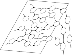
Figure 2.7.1: The problem is that most systems contain too many bubbles to fit on a normal sheet of paper.
We also understand things in a leveled way by starting with a high-level view that takes in the whole system, and then descending into the details. In systems analysis, you view the whole system by using the context diagram. (See Figure 2.7.2.)
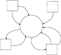
Figure 2.7.2: The context diagram shows the whole system in one bubble. The data flows around the context define the boundaries of the system.
Once you establish the context reasonably well, you reach the next stage of understanding by breaking the system into its major components. A context diagram and its breakdown are shown in Figure 2.7.3. However, the task is not always as simple as the diagram shows. Beware that the lower-level breakdown often reveals data flows that were missed at the context level. When this happens, you must then go back to make the appropriate corrections to the context diagram.
After declaring the major components and interfaces, you investigate each of them in turn. Naturally, you do this by partitioning each component into its major components and declaring the interfaces between them. In Figure 2.7.4, the high-level diagram (Diagram 0) is called the parent diagram and each of Diagrams 1 through 5 is called a child diagram.
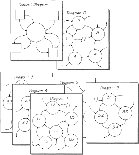
Figure 2.7.4: The top levels of the set. The context diagram declares the whole system, and Diagram 0 gives a manageable breakdown. The lower-level diagrams give a breakdown of each parent bubble at the higher level. This is called a top-down model.
The diagrams at each level show a manageable number of processes. If any of these processes is too large or too complex, then draw a lower-level diagram to partition it into still smaller and simpler pieces. You continue decomposing until you arrive at processes that are small enough to be specified.
How Much Detail at Each Level?
We began this chapter by dismissing the notion of having several hundred bubbles on one page. It’s beyond the ability of most humans to comprehend such a diagram. So just how much information can you get on one page before befuddling your reader (or yourself)?
The answer is connected to the number seven. Almost forty years ago, psychologist George Miller conducted research into the ability of humans to deal with simultaneous concepts. Miller established that at seven, plus or minus two, humans began making an intolerable number of errors.*
*George A. Miller, “The Magical Number Seven, Plus or Minus Two: Some Limits on Our Capacity for Processing Information,” The Psychological Review, Vol. 63, No. 2 (March 1956), pp. 81-97.
For completely unscientific reasons, we agree with Miller. Our experience has taught us that seven processes on one page seems to be the limit for users and analysts alike. As soon as there are seven bubbles with their associated data flows and data stores, they comfortably fill a page without being too complex. Similarly, if there are more than seven data flows into or out of a process, the process is probably too complex. We repeat, this is not scientific. We simply pretend there is a limit of approximately seven. If you also pretend the same thing, and resist building models with more than about seven bubbles per page, then your models will be easier to comprehend.
Numbering the Bubbles
Numbering the bubbles in a model is for identification purposes only. In Figure 2.7.4, note that
• The numbers do not indicate the processing sequence. They have no meaning other than identifying a specific bubble.
• Each of the child diagrams takes as its title the number of its parent. For example, bubble 1 begets Diagram 1, bubble 2 begets Diagram 2, and so on.
• The bubbles in the child diagram take the number of the parent, and each adds a decimal identifier. For example, the children of bubble 1 are numbered 1.1, 1.2, 1.3, and so on.
Identifying bubbles by a combination of the parent’s number and a decimal makes it easier to navigate around the specification. It means that from any level, both the parent diagram and the lower-level child diagrams can be readily identified. For example, to see the breakdown of a bubble, look for the diagram with the same number as the bubble. Conversely, to find the parent diagram, look for the one that contains a bubble numbered the same as the child diagram.
Functional Primitives
The little guys at the lowest level of the set are called functional primitives because they have no component parts that can be thought of as functions. The function is so simple and has no internal component that itself can be thought of as a function, so you have no need to decompose it further.
There are no internal data flows in functional primitives. The functions in a diagram are separated by data flows. If you cannot find any flows within a bubble, it is likely there are no functional subcomponents for that bubble. Remember that a data flow is a genuine collection of data elements, not just the intermediate results of a calculation that have no interest outside the bubble.
Eventually, when you have decomposed so that you can completely describe a bubble in a page or less of text, then you can stop partitioning. These one-page specifications, known as mini specifications, are fully discussed in Chapter 2.12 Mini Specifications. For the moment, remember that this is the level of the system that describes the details of the decision making, calculation, and data handling.
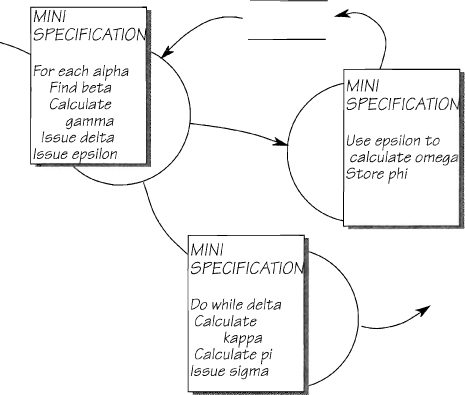
Figure 2.7.5: Functional primitives are small enough to adequately describe their processing requirements with a one-page mini specification.
Using the Imaginary Expanded Diagram
Imagine that you had the time and the patience to join all the functional primitives by their data flows. The model would then show only the processes from the lowest level of the set. This expanded diagram would look something like Figure 2.7.6.
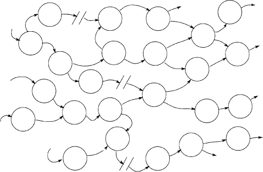
Figure 2.7.6: This expanded diagram is an imaginary diagram to illustrate the idea of joining all the functionally primitive processes.
We don’t suggest that you build such an expanded model; it negates the idea of the top-down analysis already done. Besides, there are too many problems involved. You probably couldn’t find a sheet of paper large enough to accommodate the hundreds, or possibly thousands, of bubbles. And even if you did, the resulting model would be almost impossible to read. If you could manage to read it, the effort needed to maintain this diagram would be definitely beyond your budget.
So just imagine such a diagram because you can learn something from it. The functional primitives represent the actual processes of the system. The higher levels of the model are simply convenient summaries to make the model readable. Let’s see how we can use this imaginary expanded diagram.
Repartitioning to Suit Your Purpose
The reason for having the expanded view is that the bottom level represents the actual system, and you can regroup the system’s processes to make a more logical partitioning at the higher levels. Regrouping is necessary if the original partitioning reflects the way the current system happens to be implemented. (Partitioning means breaking a system into manageable pieces, and the partitioning of many models reflects the processors and human organizations currently doing the work.) If this partitioning distorts your view of the system, you may reassemble the primitives to make a better partitioning for your model. Let’s see how this works.
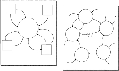
In the example (Figure 2.7.7), the partitioning in Diagram 0 was less than ideal. The large number of interfaces indicates that functions have been split between the bubbles. To correct the model, you must regroup so that functions, or closely related groups of functions, complete their processing within a bubble. When bubbles fulfill their functionality, they do not have to pass around data flows carrying incomplete results, and the interfaces between them are subsequently much narrower. To see the functionality within each bubble, you need to decompose it using a lower-level diagram. Figure 2.7.7 shows that these can be joined to make the expanded diagram.
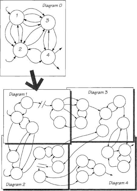
Figure 2.7.7: This model shows two levels. Note the poor partitioning in Diagram 0. The bubbles share too many interfaces, which indicates an inferior current implementation. Diagram 0 decomposes into four lower-level diagrams that are joined on the large plane at the bottom. This is the expanded diagram.
Now look for groups with closely related functionality. These groups will have narrow interfaces to the other groups. The objective is to repartition the model so that the interfaces are as narrow as possible. Figure 2.7.8 shows the groupings, and the revised Diagram 0.
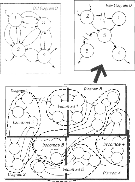
Figure 2.7.8: The analyst has regrouped the bubbles, as shown by the dotted lines. The expanded diagram is leveled upward to make the new Diagram 0.
The regrouped model reflects a more functional partitioning, and so it is a better, more rational model on which to base the design of a future system. In addition, being able to repartition or regroup the bubbles gives you some needed flexibility:
• Sometimes, your users will give you a lot of detail before you can form the big picture of Diagram 0. In this case, it is more convenient for you to model some of the middle levels before repartitioning upward to produce the top levels.
• Sometimes, you will make a bad partitioning on your first attempt at modeling the high levels. When this happens, model down to the lowest level, and then regroup upward to make a better partitioning at the top.
Remember that if you are able to decompose a bubble, you are also able to recompose one from lower-level bubbles. Decomposing and recomposing are only possible if you observe a strict convention of keeping the levels in balance with each other.
Balancing
Two levels of a model are balanced when the child diagram is processing the same data that enter and leave the parent bubble. Although the idea of balancing may seem obvious, too many projects get into difficulties because they ignore the balancing rule.
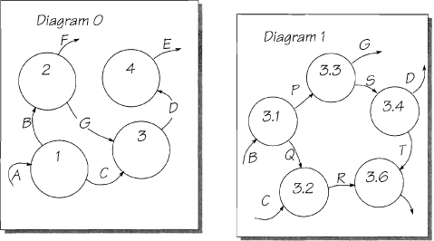
The set of diagrams shown in Figure 2.7.9 balances between the levels. The data flows in the child diagram reflect those to and from the parent bubble. Now suppose that when the analyst drew the child diagram, he included another flow (let’s call it K) leaving bubble 3.3. The diagrams are now out of balance. Why? Was the new flow overlooked at the higher level? Or is it just plain wrong and should not be part of the lower-level diagram? Whatever the reason, it must be corrected before proceeding. Similarly, if a data flow appears in the parent diagram, but not in the child diagram, this imbalance suggests that the analysis at the lower level is incomplete.
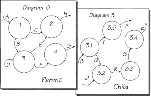
Figure 2.7.9: Two diagrams from a leveled set. Child Diagram 3 is in balance with its parent: All of the data flows into and out of the parent bubble appear in the child diagram. Similarly, the child’s external data flows—B, D, E, and F—are shown entering or leaving the parent bubble.
Balancing means that all the data flows interfacing with the parent bubble are external data flows in the child diagram. Alternatively, you could say that all external flows in the child diagram connect with the parent bubble.
If the diagrams do not balance, you cannot repartition them as we did in the example in Figure 2.7.8. Diagrams that do not balance are simply incorrect, and will not make an accurate specification for the new system.
Balancing Using the Data Dictionary
When you analyze large systems, it is sometimes convenient to bundle a number of data flows into a single flow to make the high-level diagrams easier to read. Then, when you draw the lower levels, split these bundled data flows into their components to show the functionally primitive processes.
In the example shown in Figure 2.7.10, the child diagram at first appears to be out of balance with its parent because it doesn’t show the data flow A. All data flows are defined in the data dictionary, and in this case it reveals that A is composed of R and S. As both of these flows appear in the child diagram, the model complies with the balancing rule.
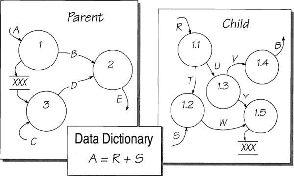
Figure 2.7.10: Parent bubble 1 shows an incoming data flow A. However, A is a bundled data flow containing the flows R and s. As the lower-level diagram shows the component flows, you must use the data dictionary to balance the model.
Balancing the Data Stores
Data stores in leveled models have their own balancing rule: Show data stores at the highest level where they are used by more than one bubble and at every relevant lower level. When you decompose a process that accesses a data store, that store must appear in the lower levels if the diagrams are to remain in balance. When only one bubble in the diagram accesses a store, it looks a little odd; however, it is necessary if your reader is to make sense of the low-level diagrams.
Just as you can group data flows in higher-level diagrams, you can also have composite data stores. When there are many data stores in the system, some analysts prefer to collect them into a composite store, such as an “accounts database” or “operations file,” and then break them into smaller data stores in the child diagrams. The advantage of this approach is that the decomposed stores show the precise data usage of the low-level processes.
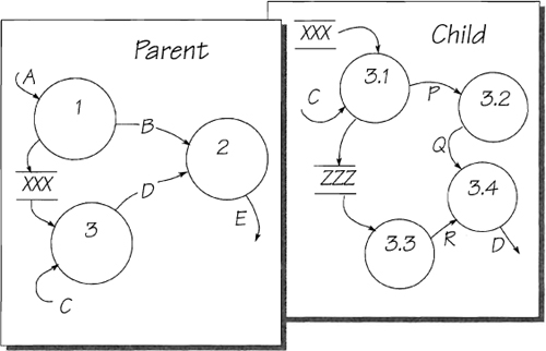
Figure 2.7.11: The parent diagram shows two bubbles sharing the data store xxx. It also appears in the child diagram as input to bubble 3.1. The child diagram reveals data store zzz, which was hidden inside bubble 3 at the higher level.
Summary
You can use leveling to control the number of bubbles you wish to show in any one diagram. You also use leveling to present a top-down model of the system. You would like your end result to be a specification that is organized in a top-down manner because it is easier to control and to check for consistency and completeness. Although you can think of analysis as a top-down activity, it is rarely done this way. The reason is that you typically get the system information in a random manner, as the users supply it. As you interview different people in an organization, they give you information at different levels. To cope with this situation, you must feel comfortable about building your models at any level, and decomposing and recomposing to make the most logical partitioning of the system.
It is perfectly acceptable for you to draw a data flow diagram without knowing precisely at which level the diagram fits into the system model, and you may decompose and recompose several times before you establish it at the correct location. There is nothing wrong with that; it is just part of the craft of systems analysis. You must become comfortable with the idea of working top-down, bottom-up, middle-up, or middle-down.
The balancing rule ensures the model’s integrity by proving that each child diagram is a faithful decomposition of the parent. The high-level models act as a guide to the details in the lower-level models.
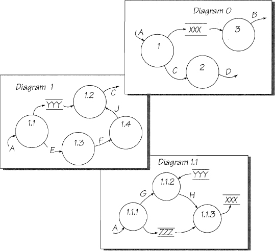
Exercise 1: Find the Leveling Problems
There are some problems with the leveling in the set of diagrams shown in Figure 2.7.12. Highlight all the errors you find. Ignore the single-letter names in this and subsequent models. They are used only to simplify the diagrams.
Exercise 2: Balancing Data Stores
The set of diagrams in Figure 2.7.13 has some problems with the data stores. Highlight the errors and tell why you think each one is wrong.
Exercise 3: Draw the Parent Bubble
Figure 2.7.14 shows a child diagram. Draw the parent bubble. Group the data flows to make the parent as readable as possible, and say what data make up any new flows introduced into your new diagram.

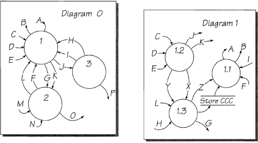
Exercise 4: Repartition the Model
Here is a leveled set of diagrams, but they are not very useful. Diagram 0 is badly partitioned. Can you make the model more useful by repartitioning in some way?
![]() Easiest: You now have all the information you need about data flow models. But when you build a model, it needs a viewpoint. One that you will find useful as you continue to explore the Piccadilly system is the current physical viewpoint. We discuss this in your next chapter, 2.8 Current Physical Viewpoint.
Easiest: You now have all the information you need about data flow models. But when you build a model, it needs a viewpoint. One that you will find useful as you continue to explore the Piccadilly system is the current physical viewpoint. We discuss this in your next chapter, 2.8 Current Physical Viewpoint.
![]() More Difficult: This chapter is not part of your trail; your next chapter is 2.8 Current Physical Viewpoint.
More Difficult: This chapter is not part of your trail; your next chapter is 2.8 Current Physical Viewpoint.
![]() Most Difficult: This was not intended reading for you, and Chapter 1.4 The Piccadilly Organization is the best destination for you.
Most Difficult: This was not intended reading for you, and Chapter 1.4 The Piccadilly Organization is the best destination for you.
![]() Promenade: We didn’t intend you to be here, but hope that you found leveling interesting. Turn now to Chapter 2.8 Current Physical Viewpoint.
Promenade: We didn’t intend you to be here, but hope that you found leveling interesting. Turn now to Chapter 2.8 Current Physical Viewpoint.