C h a p t e r 1 5
Module 7—Using
Everyday Statistics
Module 7 covers some very basic concepts of statistics that may be helpful when making decisions. It should be used with the multiple-day program schedules. Special suggestion with this module: If your boss is going to walk by the training room and see people playing with cards and dice, perhaps you should first warn him or her about the relevance of the exercise.
Training Objectives
After completing this module, the participants should be able to
- define probability, using everyday examples
- use the concept of probability to explain gambling situations
- explain the process and uses of sampling data related to decision making.
 Module 7 Time
- Approximately 1.5 hours
Note: This schedule includes time for a quick review at the start and a learning check at the end.
Materials
- Attendance list
- Pencils, pens, and paper for each participant
- Whiteboard or flipchart and markers
- Name tags or name tents for each participant
- Worksheet 15–1: Probability, Combinations, and Permutations
- Worksheet 15–2: Statistical Techniques
- Computer, screen, and projector for displaying PowerPoint slides; alternatively, overhead projector and overhead transparencies
- PowerPoint slide program (slides 15–1 through 15–23)
- This chapter for reference or detailed facilitator notes
- Optional: music, coffee, or other refreshments. Also, having calculators available for participants will be useful (one per subgroup or one per participant).
- Several decks of cards and several pairs of dice.
Module Preparation
Arrive ahead of time to greet the participants and make sure materials are available and laid out for the way you want to run the class. Turn on and test computer equipment.
NOTE ABOUT THIS MODULE: MAKE IT FUN
This module can be intimidating to many participants (and to a few trainers). But the worksheets, PowerPoint slides, and trainer’s notes will encourage you to make this module fun by drawing on the intuitive understanding that people have about statistics (though they might not have brought it to the conscious surface previously).
Observe the skill levels and levels of comfort of your participants and adjust your presentation accordingly. This session should not be lecture-only. For the exercises, you may want to ease any pressure by mixing groups with skilled and unskilled people and by demonstrating steps on the whiteboard or flipchart item by item.
Work on the concepts one at a time (that’s how the slides are designed). Rather than presenting the concepts as a solid block, insert the slides with quotes and promote discussion between the concepts. You may also want to split up the worksheet into several parts and give out one problem at a time.
Sample Agenda
| 0:00 | Welcome the class. |
| Have slide 15–1 on the screen as participants arrive. | |
| 0:05 | Exercise. |
| Hand out the card decks and dice, and suggest that people discuss gambling. | |
| 0:20 | PPT Presentation and worksheets. |
| Begin with slide 15–2 (objectives) and proceed through slide 15–21. See notes in the PowerPoint file and in the Trainer’s Notes. Distribute Worksheet 15–1: Probability, Combinations, and Permutations. | |
| See notes below on preparation of worksheets for this module. | |
| Move among participants to keep them on task. | |
| It’s OK for participants to discuss answers with others. | |
| 1:15 | Practice. |
| Continue work on Worksheet 15–1: Probability, Combinations, and Permutations and distribute Worksheet 15–2: Statistical Techniques. | |
| 1:25 | Wrap-up. |
| Show slide 15–22. Review the module 7 objectives with the class. | |
| Ask for questions and concerns. | |
| Check for learning (questions can be in oral or printed format). | |
| Show slide 15–23. Dismiss the class. |
Trainer’s Notes
8:00 a.m. Welcome (10 minutes).
Show slide 15–1 as participants arrive.
Take care of housekeeping items.
Distribute card decks and dice. Encourage the participants to talk among themselves about the idea of gambling.
8:10 a.m. Probability (40 minutes).
Show slide 15–2 and preview module 7 topics.
Note: This module is designed so that the worksheet exercises are intermixed with the PowerPoint presentation. Allow about 50 to 60 minutes to complete slides 15–2 through 15–19. You can also include an optional short (5-minute) break at a convenient point during that time. If you prefer to do all of the worksheet exercises at the end, you’ll need to adjust the PowerPoint slides accordingly and not distribute the worksheets until you’ve completed slide 15–21.
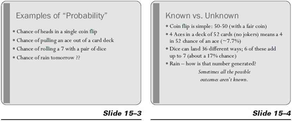
Show slide 15–3. Go over the probability examples on the slide with the participants or have them work alone on the calculations.
Show slide 15–4.
Go over the answers with the class. The first two are pretty easy, but you may want to illustrate the third. Go to the board and write out the calculation. Using two different color markers (red and black, for example), write out two columns of numbers: one through six, one red column and one black column. Then match up the numbers in the red column and the black column that add to seven. Circle the combinations that add to seven: R1/B6; R2/B5; R3/B4; R4/B3; R5/B2; R6/B1. Six different combinations add up to seven and 30 combinations don’t. So the odds of rolling a seven are six to 30, or one to five.
Ask the learners why the final (the rain forecast) example is different.
Explain that the last example is different because there are other unknown factors at work. The probability for rain is based on a computer model, probably using artificial intelligence software, which takes the atmospheric conditions projected for the next day and manipulates it to compare with similar conditions in the past and how often it rained under those conditions. Or, in the small towns it may be that six out of 10 of the guys at Mel’s coffee shop have back pain, so it works out at 60 percent chance of rain.
Show slide 15–5, and discuss how the past is not a true predictor of the future.
Show slide 15–6. In addition to reading the text of the slide, explain the concept of an exponent. (1/2)3 means that the number (one-half in this case) multiplied by itself the number of times shown in the exponent (three, in this case). So 1/2 × 1/2 × 1/2 = 1/8.
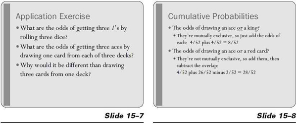
 Show slide 15–7.
Allow a minute or two for the participants to answer the three questions on the slide. The answers to the questions:
(1) 1/6 × 1/6 × 1/6 = 1/216 or odds of 216 to one.
(2) Drawing from three decks would be calculated as (4/52)3 = 4/52 × 4/52 × 4/52 = one out of 2,197.
(3) Drawing three aces from one deck (without replacing the card drawn) would be calculated as 4/52 × 3/51 × 2/50 = 0.000181 or about 1 out of 5525.
Show slide 15–8. This slide will be self-explanatory for many participants, but be prepared to explain “mutually exclusive.” And be prepared to explain “4/52 + 26/52 – 2/52 = 28/52.” Four out of 52 cards are aces, 26 out of 52 cards are red, and two cards are red aces, so those two have been double counted and therefore two needs to be subtracted. They are not mutually exclusive because a card can be both red and an ace.
 Show slide 15–9. Distribute Worksheet 15–1: Probability, Combinations, and Permutations. Allow no more than five minutes for the first part of the worksheet.
Now, you have choices to make about how you present the next exercises.
- Either allow participants to work together, or change the slide if you don’t want them to work together.
- Present all the questions on the worksheet at once, or split up the worksheet and distribute the parts as you go along.
After distributing Worksheet 15–1, allow time for participants to solve the first question: (1) What are the odds of getting four heads and no tails out of flipping four coins? Then show the next slide.
Show slide 15–10.
Discuss the quote with the participants.
Direct participants to answer the second question on Worksheet 15–1. (2) What is the probability of drawing an ace and a black king on two consecutive draws from the same deck without replacing cards?
After allowing time for participants to calculate the answer, put the answer on the whiteboard or flipchart.
On the first draw, chances are four out of 52 that you will draw an ace; on the second draw, your chances are two out of 51 that you will draw a black king. Therefore, your chances of drawing an ace and a black king in two draws is the product of those two multiplied, or (4/52) × (2/51) = 2/663.
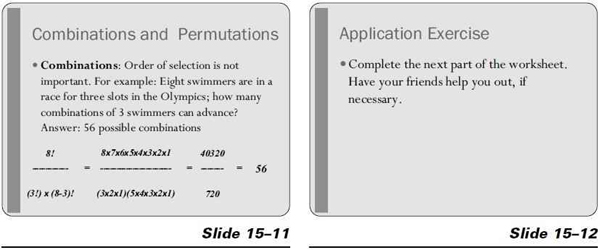
Show slide 15–11.
Explain the “!” notation in math. This is called “factorial” and means any integer multiplied by each integer less than itself. So, 4! = 4 × 3 × 2 × 1 = 24.
Be prepared to discuss why order of selection is not important for combinations and why it is important in calculating permutations.
Show slide 15–12.
Direct participants to answer the third question on Worksheet 15–1. (3) Five different color balls are in a box. If you draw out three at random, how many different combinations can be created?
After allowing time for participants to calculate the answer, put the answer on the board or flipchart.
(5!) ÷ (3!)(5 − 3)! = (5 × 4 × 3 × 2 × 1) ÷ (3 × 2 × 1)(2 × 1) = 120 ÷ 12 = 10
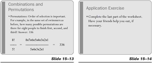
Show slide 15–13. Review the material on the slide.
Show slide 15–14.
Direct participants to answer the fourth question on the Worksheet 15–1: (4) How many different ways can you sequence the words “love,” “honor,” and “obey”?).
After allowing time for participants to calculate the answer, put the answer on the whiteboard or flipchart.
3! ÷ 1! = (3 × 2 × 1) ÷ (1) = 6
love, honor, obey
love, obey, honor
honor, love, obey
honor, obey, love
obey, love, honor
obey, honor, love
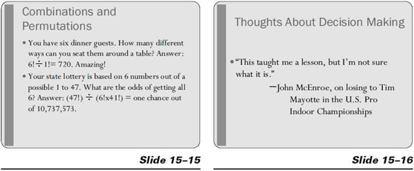
Show slide 15–15. Read the slide or let the participants read it. It shows additional ways that these principles can be applied.
Show slide 15–16. This John McEnroe quote is just to get a smile and reduce some of the tension that working with statistics usually causes.
8:50 a.m. Break (Optional) (5 minutes).
Usually people need one by now. Keep it short.
8:55 a.m. Data Sampling (20 minutes).
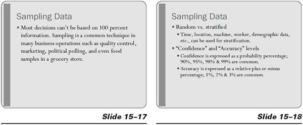
Show slide 15–17.
Explain that the next section is about data sampling. We don’t have time for a comprehensive treatment of the subject of sampling. Like the rest of this training program, we hope that you’ll use sampling as a tool for gathering data to help with your decision-making process when it’s appropriate. If any of you actually needs to design a sampling study, you should contact someone who understands it in greater depth than provided here.
We see sampling results in the news every day from political polls. For years, USA Today has featured the results of sampling and polling. Somewhere in your organization at this moment, there is sampling taking place. Where is that likely to be? (Quality control and marketing are likely answers.) Note: See if you can find some recent relevant examples to use - political polls or other polls show up almost every day in newspapers. There may also be some from your company experience.
We’ll discuss how many samples you need to become reasonably certain of accuracy. The size of the sample should be determined by the nature of what you’re sampling. In the grocery store, you may only need one taste of Harry’s Horribly Hot Jalapeno Dip to decide whether or not you want to buy it. On the other hand, Harry probably needs to sample quite a few cans of his production to ensure that the quality is staying where he wants it. He also needs to sample a number of customers to see if the recipe needs to be changed. He probably should not change it based on just one person’s opinion.
Show slide 15–18.
Introduce the concept of sampling. For sampling to be useful, it must truly represent the entire population from which it is taken. For example, a poll to determine political attitudes of the country could not be conducted only in Boston or only in San Diego. To ensure the representativeness of a sample, you must first know something about the population.
Populations that are truly homogeneous can be sampled in any manner. Probably very few truly homogeneous populations exist, but there are many in which the differences are not significant or not related to the variable being measured. Random samples can be taken at any time, any place, in any order. All that’s necessary is to get a sufficient quantity of samples.
In many cases, however, stratified samples are necessary. To stratify means to ensure that there is a representative mix of the population within the sample. Let’s use an example: if you’re sampling a production process, you need to sample across all time periods and job categories. If you sampled only mornings or materials handlers, your information would only be usable for that group at that time.
Common categories (or variables) for stratification include
Time. Commonly, an equal number of samples is taken each hour of operation.
Location. All locations of operation should be appropriately represented in the sample.
Machine. Products made on various machines need to be included in the sample to ensure overall accuracy.
Worker. Work done by each worker needs to be included in the sample.
Demographic data. Public opinion surveys need to include representative mixes of various ages, races, employment categories, income levels, and so forth.
Other factors. Any categories that could potentially provide different data than the rest of the sample need to be proportionately included.
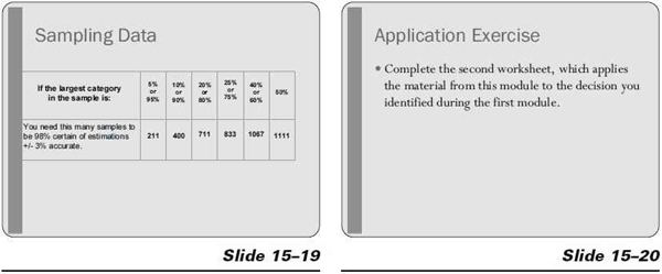
You can determine through statistical means how accurately and with what level of confidence a sample represents its population. An easy-to-remember number, which is a standard in the sampling business, is 1111. That’s the largest number of samples you’ll ever need to take out of a population to be 98 percent certain that your sample is within plus or minus 3 percent of the actual population. Depending on what you’re sampling, you may need dramatically fewer samples. Sampling theory is the subject of entire textbooks. The only concern we have is to explain how many samples are needed to reach a given level of accuracy. In general, the more samples (properly taken samples, at least), the greater the accuracy. The level of accuracy is expressed in terms of plus or minus a certain percent accuracy at a specific level of confidence. For example, we might be 98 percent confident that our sample is plus or minus 3 percent accurate.
The first number is a probability (98 percent of the time under these conditions), and the other is a statement of relativity (the figures we have developed from our sample are within 3 percent of the actual population). The two terms work in tandem. Probability will increase (get higher) as the variation from population increases. For certain samples, it might be equally true to say that we are 95 percent confident of plus or minus 3 percent accuracy, or that we are 99 percent confident of plus or minus 10 percent accuracy.
You must start with the confidence level you wish to have. 90, 95, 98, and 99 percent are common choices in statistics. Given that confidence level, you determine the accuracy level based on the number of samples and the ratio of the samples in the largest category to the total samples. The table on the next slide indicates the samples needed for 3 percent accuracy at 98 percent confidence.
Show slide 15–19.
9:15 a.m. Application Exercise (10 minutes).
Show slide 15–20. Distribute Worksheet 15–2: Statistical Techniques and allow participants to complete it. Move among them to keep them on task. This worksheet continues the pattern of building on decisions identified in module 1.
Show slide 15–21.
Review the Lovin’ Spoonful quote with the class. Have a sing-along, if you wish. If you’re using music with your lesson design, this song might be a good choice.
9:25 a.m. Module 7 Summary (5 minutes).
Show slide 15–22, and review the key points of the module. Use the following questions, as desired.
 LEARNING CHECK QUESTIONS
You can use the learning check questions and answers in oral or printed form.
Discusssion Questions
- Does an honest deck of cards represent a known or an unknown universe?
Answer: a known universe - Why is sampling a good idea in collection of information?
Answer: It’s usually cheaper and faster than polling the entire population, especially if you have an unknown population or large known population of possibilities. - What steps can improve the accuracy of the results of a survey to collect primary data on product preference?
Answer: (1) Increase the number of samples, (2) ensure the sample is properly stratified to reflect the target population and (3) pretest questions for reliability and validity. - A legal game at the county fair allows you to put $1 on a number, spin a wheel with 20 numbers on it, and win $10 if the wheel stops at your number. List and explain three or four things that would influence your decision whether or not to play this game.
Possible answers: (1) your attitude toward gambling, (2) your need for $1 (can I afford to lose it?), (3) your tolerance for risk, and (4) the odds of winning, and so forth.
Multiple Choice Questions
- The best example of probability that involves a known universe is
a. Predicting which candidate will win the election
b. Playing a game of poker (answer)
c. Guessing the number of beans in a jar
d. Buying a used car that won’t break down. - Which of the numbers below is more likely than others to result from a single roll of a pair of fair dice?
a. 2
b. 6 (answer)
c. 10
d. 12
9:30 a.m. Thank You for Your Attention.
Show slide 15–23. Edit slide to show relevant information.
Worksheet 15–1
Calculate the following probabilities:
1. What are the odds of getting four heads and no tails out of flipping four coins?
2. What is the probability of drawing an ace and a black king on two draws from the same deck (without replacing cards)?
Calculate the following combination:
3. Five different color balls are in a box. If you draw out three at random, how many different combinations can be created?
Calculate the following permutation:
4. How many ways can sequence the words “love,” “honor,” and “obey”?
Answers (Note: Do not print the answers on the same page as the questions.)
(1/2)4 = 1/16 or one out of sixteen
HHHH, HHHT, HHTT, HTTT
HHTT, HHTH, HTHH, HTHT
THHH, THHT, THTT, TTTT
TTHH, TTTH, THTT, THTH
First-draw chances are four out of 52; second-draw chances are two out of 51. Therefore the total chance is the product of those two multiplied, or (4/52) × (2/51) = 2/663
(5!) ÷ (3!)(5 − 3)! = (5 × 4 × 3 × 2 × 1) ÷ (3 × 2 × 1)(2 × 1) = 10
3! ÷ 1! = (3 × 2 × 1) ÷ (1) = 6
love, honor, obey
love, obey, honor
honor, love, obey
honor, obey, love
obey, love, honor
obey, honor, love
© 2010 Decision-Making Training, American Society for Training & Development
Worksheet 15–2
Restate the decision that you are working on for this training program.
What data is required to treat your decision with statistics?
What sampling data might be collected and how would you collect it?
Will random samples do, or do you need to stratify the data in any way? If so, how?
© 2010 Decision-Making Training, American Society for Training & Development