
Chapter 17. Cloth Simulation in the Bullet Physics SDK
By Lee Howes and Benedict R. Gaster
The Bullet Physics SDK is a widely used, open-source, collision detection, rigid-body and soft-body dynamics library available for free, for a wide range of platforms, under the zlib License. It supports discrete and continuous collision detection on concave and convex meshes as well as basic primitives. Bullet has a fast and stable rigid-body dynamics constraint solver, vehicle dynamics, character controller, and a range of constraint types. More interestingly for our purposes, Bullet includes soft-body dynamics supporting cloth, rope, and deformable volumes with two-way interaction with rigid bodies.
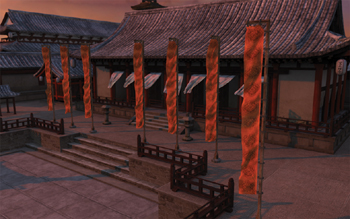
In this chapter, we describe an implementation of some of the basic features of soft-body dynamics into an OpenCL accelerated framework. This OpenCL code is released in the 2.77 version of the Bullet SDK and is available for download from http://bulletphysics.org. Figure 17.1 shows flags simulated using the Bullet SDK’s cloth implementation in AMD’s Samari demo.1
Figure 17.1 AMD’s Samari demo, courtesy of Jason Yang
An Introduction to Cloth Simulation
There are many ways of simulating soft bodies. Finite element methods offer a physically accurate approach by breaking down the soft body into elements, often tetrahedra, over which partial differential equations are solved for the stresses in each element. Shape matching applies a penalty to parts of a model based on their distance from some optimal position, with the effect of driving the object toward its original shape. Mass/spring models construct the soft body from a set of masses connected by weightless springs that apply forces to the masses based on their compression or extension from rest length; that is, they obey a variant of Hooke’s law.
The simulation method used in Bullet is similar to a mass/spring model (see Figures 17.2 and 17.3), but rather than applying forces to the masses, it applies position and velocity corrections based on the work of Thomas Jakobsen, presented at GDC 2001 in a talk entitled “Advanced Character Physics.”
Figure 17.2 Masses and connecting links, similar to a mass/spring model for soft bodies
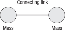
Figure 17.3 Creating a simulation structure from a cloth mesh
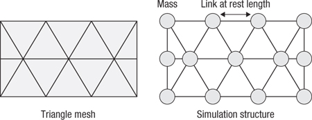
The input to the simulation is a mesh representing the body to simulate. In general, this is a clothlike structure: two-dimensional in concept, mapped to three-dimensional space. From this mesh we create simulation masses at each vertex and simulation links for the connecting mesh links. The initial length of the links based on the positions of vertices in the mesh gives the rest length. The structure offered by the rest length defines the shape that, independent of external forces such as gravity, the cloth will maintain. These links have a relatively high strength for most cloth as such material does not stretch significantly under the application of day-to-day forces.
The astute reader may notice that while the mesh links alone may be enough to maintain a rigid structure for a three-dimensional body if constructed from a tetrahedral mesh, for a surface there is insufficient structure. Without any form of angle constraint on a vertex there is no resistance to folding over a vertex: two vertices linked from a central vertex are free to move relative to each other as long as their individual distances from the central vertex do not change. This motivates the need for an additional type of link in the structure that is usually given a lower resistance to displacement from its rest length (see Figure 17.4).
Figure 17.4 Cloth link structure
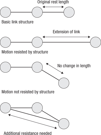
An additional link spanning a central vertex is necessary to maintain the relationship between nodes that are not directly connected. This allows us to maintain three-dimensional structure in the cloth and resist bending.
At this core of the simulation these types of links are treated no differently; however, from the point of view of creation of the input we cannot create the bend links directly from the mesh. Instead we can infer a link across every triangle boundary and add this to the simulation data structure. The result is that our original simulation mesh becomes something like what is shown in Figure 17.5.
Figure 17.5 Cloth mesh with both structural links that stop stretching and bend links that resist folding of the material
In two dimensions repeatedly solving this mesh gives us clothlike behavior, controlled by strengths assigned to links and masses assigned to nodes. In three dimensions, and without the need for bend links, more varied soft-body structures can be constructed.
Simulating the Soft Body
Simulating the mesh involves performing an iterative relaxation solver over each of the links. Each time step performs an iterative solve first of velocities of nodes in the mesh, obtaining velocity corrections for each node. It then updates estimated positions from the velocities and iteratively computes position corrections. In both the velocity and position updates the solver computes new values for the particles at either end of a given link based on the masses of the particles, the strength of the link, and its extension or compression.
We can picture this solver’s application to simulation in a simple one-dimensional ropelike structure as shown in Figure 17.6(a). In the figure we see a series of masses connected by springlike links. If we apply a force such as gravity, a motion resulting from some sort of collision, or some user input to the rope, we may move one of the vertices from rest as in Figure 17.6(b).
Figure 17.6 Solving the mesh of a rope. Note how the motion applied between (a) and (b) propagates during solver iterations (c) and (d) until, eventually, the entire rope has been affected.
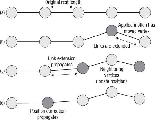
As we move to Figure 17.6(c), we apply the first iteration of the solver. This applies the motion resulting from the distortion of the mesh seen in the extended links in Figure 17.6(b) such that the neighboring vertices’ positions are updated. In Figure 17.6(d) a similar process propagates the motion through to another vertex. We see this distortion propagate through a complex mesh in complicated patterns as the motion of one vertex affects multiple other vertices; eventually, if we iterate for long enough, we should reach a stable state.
Roughly the algorithm follows the following structure where k is a constant link stretch factor and linkLengthRatio is the reciprocal of the square of the link length times the sum of the masses on the link:
for each time step
Prepare links
for each velocity iteration
for each link in mesh
(velocity0, inverseMass0) = linkStart
(velocity1, inverseMass1) = linkEnd
float3 velocityDifference = velocity1 – velocity0;
float velAlongLink = dot( linkVector, velocityDifference );
float correction = -velAlongLink*linkLengthRatio*k;
velocity0 -= linkVector*k*inverseMass0;
velocity1 += linkVector*k*inverseMass1;
Estimate position corrections from velocities
for each position iteration
for each link in mesh
(position0, inverseMass0) = linkStart
(position1, inverseMass1) = linkEnd
float3 vectorLength = position1 - position0;
float length = dot(vectorLength, vectorLength);
float k = ( (restLengthSquared - len) /
(massLSC*(restLengthSquared+len)))*kst;
position0 -= vectorLength * (k*inverseMass0);
position1 += vectorLength * (k*inverseMass1);
The idea of these repeated iterations is to converge on a stable solution of the system of equations comprising the mesh structure. If we were aiming for a stable solution, we would iterate both the velocity and the position solver until the system converged completely.
For the purposes of real-time physics simulation, however, two other factors come into play:
• Performance predictability is more stable than achieving a fully stable situation.
• The time-step iteration loop also affects convergence. To an extent the convergence carries over from one time step to the next if the change created at a given time step is not too significant.
To this end a simulation used in practice will usually set a fixed number of iterations, chosen both to achieve a reasonable level of convergence and to support the required frame rate.
Executing the Simulation on the CPU
As is often the case, performing the simulation on the CPU is a relatively simple process. A high degree of code structure can be maintained to ensure good readability and flexibility. For each individual soft body we can run the solver code across all the links in the soft body.
The following code represents the position solver for a single soft-body object. m_c0 and m_c1 are per-link constants that are precomputed. The velocity solver code is similar; we shall ignore that and the simple per-vertex update loops for the rest of this discussion.
void btSoftBody::PSolve_Links(
btSoftBody* psb,
btScalar kst,
btScalar ti)
{
for(int i=0, ni = psb->m_links.size(); i < ni; ++i)
{
Link &l=psb->m_links[i];
if(l.m_c0>0) {
Node &a = *l.m_normal[0];
Node &b = *l.m_normal [1];
const btVector3 del = b.m_position - a.m_position;
const btScalar len = del.length2();
const btScalar k =
((l.m_c1 - len)/(l.m_c0 * (l.m_c1 + len)))*
simulationConstant;
a.m_x -= del*(k*a.m_inverseMass);
b.m_x += del*(k*b.m_inverseMass);
}
}
}
For each soft body we can tweak the set of solver stages we wish to execute, the number of stages, and so on. For example, we might want to execute five velocity iterations and ten position iterations for a very large soft body where propagation of forces through the mesh would be slow.
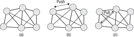
Note that this loop executes over data in place. By updating in place the result of computing the effect on a vertex of a single link is used to compute the effect of a second link on both that same vertex and its connected neighbor. This approach is often known as Gauss-Seidel iteration. This has important behavioral characteristics that apply when we look at the GPU implementation of the solver. We can see how this behaves in Figure 17.7.
Figure 17.7 The stages of Gauss-Seidel iteration on a set of soft-body links and vertices. In (a) we see the mesh at the start of the solver iteration. In (b) we apply the effects of the first link on its vertices. In (c) we apply those of another link, noting that we work from the positions computed in (b).
One aspect that should be clear from this loop, and indeed from the Gauss-Seidel iteration it uses, is that it is not trivially parallelizable by a compiler. There is an inter-iteration dependence, and as such a trivial parallelization of this loop will lead to subtle differences in behavior, and possibly incorrect results.
Changes Necessary for Basic GPU Execution
The first thing to note is that the large amount of parallelism in the OpenCL programming model means that unless soft bodies are very large, solving soft bodies individually is inefficient because each soft body has too little parallelism during an iteration of any of its solvers to fully use the device. As a result, the first thing we want to do is solve multiple soft bodies simultaneously, allowing their combined computation needs to fill the entire device. In the Bullet solver this means that soft-body data is moved into single large arrays, indexed by values in the individual soft-body objects. These entire arrays are moved onto the GPU, operated on, and if necessary moved back to the host memory.
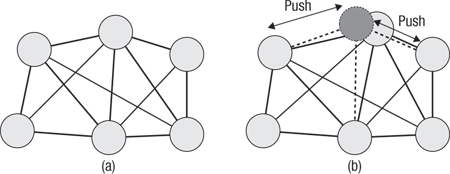
Unfortunately, performing the original CPU calculation in parallel over all links in all soft bodies in this fashion produces incorrect results. Looking back at Figure 17.5, we can see that as each link is solved, the positions or velocities of the vertices at either end are updated. If we perform the computations in parallel, they attempt to produce a result along the lines of what is shown in Figure 17.8, but applied to every mass rather than only the one shown.
Figure 17.8 The same mesh as in Figure 17.7 is shown in (a). In (b) the update shown in Figure 17.7(c) has occurred as well as a second update represented by the dark mass and dotted lines.
We can solve this in various ways. Many simulations choose to use a Jacobi-style loop, which would run for each vertex and update that vertex based on the position updates the surrounding links would apply, or, more commonly in such simulations, based on the sum of forces applied by the surrounding links. This type of simulation is easier to implement because it can double-buffer the computation, but the cost is that propagation of updates through the soft body tends to be slower, and in a position- and velocity-based simulation such as that used here, momentum is not conserved; that is, the updates introduce error. This error can be reduced through damping but at a cost for the simulation.
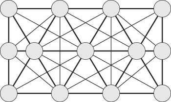
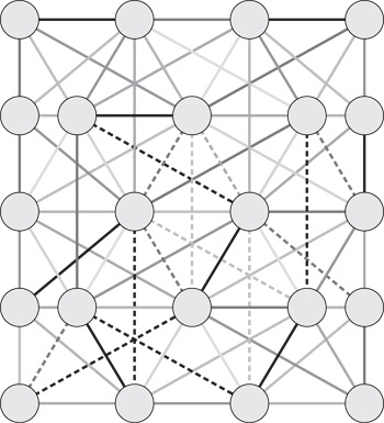
The alternative approach that we use here is to perform a graph coloring of the mesh. That is, we choose a batch number for each link such that any two links in the mesh that share a vertex will not be in the same batch. This requires a large number of batches that will be based on the complexity of the interconnections in the mesh; indeed it will be equal to the valence of maximum note in the mesh. In the mesh seen in Figure 17.5 that would be 5. The vertex in the center of each row is connected to all five other vertices. In the mesh seen in Figure 17.9 we can see an example of a minimum coloring that requires 12 colors.2 For a more complicated mesh this would be a substantially higher number.
Figure 17.9 A mesh with structural links taken from the input triangle mesh and bend links created across triangle boundaries with one possible coloring into independent batches
To implement this on the GPU we first sort the link data into batches. The simplest approach is the following:
for each link:
color = 0
Here, color is used by any other link connected to either vertex connected to this link:
color = next color
linkBatch = color
This batching operation need only be performed once unless the mesh changes. In a simple implementation the mesh need not change, and adapting for tearing is more efficiently dealt with by disabling links than by rebatching.
To execute we iterate over the batches, performing one parallel OpenCL dispatch for each, knowing that each batch is entirely parallel. Where before we called solveConstraints and then inside that PSolve_Links on a single soft body, now we call solveConstraints over an entire set of soft bodies with the following loop:
for(int iteration = 0;
iteration < m_numberOfPositionIterations;
++iteration ) {
for( int i = 0;
i < m_linkData.m_batchStartLengths.size();
++i ) {
int startLink = m_linkData.m_batchStartLengths[i].start;
int numLinks = m_linkData.m_batchStartLengths[i].length;
solveLinksForPosition( startLink, numLinks, kst, ti );
}
}
Note that solveLinksForPosition is being called to act on a range of links within a given precomputed batch. This set of batches is computed using the algorithm discussed previously. The kernel is called using the following code that sets up the OpenCL launch and executes:
void btOpenCLSoftBodySolver::solveLinksForPosition(
int startLink,
int numLinks,
float kst,
float ti)
{
cl_int ciErrNum;
ciErrNum = clSetKernelArg(
solvePositionsFromLinksKernel,
0,
sizeof(int),
&startLink);
ciErrNum = clSetKernelArg(
solvePositionsFromLinksKernel,
1,
sizeof(int),
&numLinks);
ciErrNum = clSetKernelArg(
solvePositionsFromLinksKernel,
2,
sizeof(float),
&kst);
ciErrNum = clSetKernelArg(
solvePositionsFromLinksKernel,
3,
sizeof(float),
&ti);
ciErrNum = clSetKernelArg(
solvePositionsFromLinksKernel,
4,
sizeof(cl_mem),
&m_linkData.m_clLinks.m_buffer);
ciErrNum = clSetKernelArg(
solvePositionsFromLinksKernel,
5,
sizeof(cl_mem),
&m_linkData.m_clLinksMassLSC.m_buffer);
ciErrNum = clSetKernelArg(
solvePositionsFromLinksKernel,
6,
sizeof(cl_mem),
&m_linkData.m_clLinksRestLengthSquared.m_buffer);
ciErrNum = clSetKernelArg(
solvePositionsFromLinksKernel,
7,
sizeof(cl_mem),
&m_vertexData.m_clVertexInverseMass.m_buffer);
ciErrNum = clSetKernelArg(
solvePositionsFromLinksKernel,
8,
sizeof(cl_mem),
&m_vertexData.m_clVertexPosition.m_buffer);
size_t numWorkItems = workGroupSize*
((numLinks + (workGroupSize-1)) / workGroupSize);
ciErrNum = clEnqueueNDRangeKernel(
m_cqCommandQue,
solvePositionsFromLinksKernel,
1,
NULL,
&numWorkItems,
&workGroupSize,0,0,0);
if( ciErrNum!= CL_SUCCESS ) {
btAssert( 0 &&
"enqueueNDRangeKernel(solvePositionsFromLinksKernel)");
}
} // solveLinksForPosition
The GPU executes an OpenCL kernel compiled from the following code:
__kernel void
SolvePositionsFromLinksKernel(
const int startLink,
const int numLinks,
const float kst,
const float ti,
__global int2 * g_linksVertexIndices,
__global float * g_linksMassLSC,
__global float * g_linksRestLengthSquared,
__global float * g_verticesInverseMass,
__global float4 * g_vertexPositions)
{
int linkID = get_global_id(0) + startLink;
if( get_global_id(0) < numLinks ) {
float massLSC = g_linksMassLSC[linkID];
float restLengthSquared = g_linksRestLengthSquared[linkID];
if( massLSC > 0.0f ) {
int2 nodeIndices = g_linksVertexIndices[linkID];
int node0 = nodeIndices.x;
int node1 = nodeIndices.y;
float3 position0 = g_vertexPositions[node0].xyz;
float3 position1 = g_vertexPositions[node1].xyz;
float inverseMass0 = g_verticesInverseMass[node0];
float inverseMass1 = g_verticesInverseMass[node1];
float3 del = position1 - position0;
float len = dot(del, del);
float k = ((restLengthSquared -
len)/(massLSC*(restLengthSquared+len)))*kst;
position0 = position0 - del*(k*inverseMass0);
position1 = position1 + del*(k*inverseMass1);
g_vertexPositions[node0] = (float4)(position0, 0.f);
g_vertexPositions[node1] = (float4)(position1, 0.f);
}
}
}
In this version of the code, for each batch we are enqueuing an OpenCL kernel that will have to wait for completion of the previously enqueued instance before it can execute. Each kernel dispatch takes some amount of time to prepare for execution: the GPU must be set up, register values passed, bus transactions enacted, and so on. We can infer from this that as we increase the number of kernel dispatches, we increase the amount of time it takes to execute not only in GPU time but also in CPU time to manage that GPU execution.
In addition to CPU overhead, as we increase the number of dispatches without increasing the amount of work, it should be clear that the work per dispatch becomes smaller. There will always be a point at which the work per dispatch is low enough to not fully occupy the GPU, or at least not occupy the GPU for long enough to overlap with any of the CPU overhead that could be overlapped.
Given that small enough workloads and large enough numbers of dispatches increase CPU overhead, it is possible for an algorithm to eventually become dispatch-bound. The next section discusses one approach that we can use to deal with this. In addition, we take into account the SIMD nature of GPU hardware to increase efficiency further.
Two-Layered Batching
The first thing to look at is why we need so many batches. In Figure 17.9 we saw a coloring of the graph that shows that the number required was at least equal to the highest vertex valence in the graph. Clearly in having connections to neighboring vertices and to distant vertices with the addition of bend links (the structure of which depends on the required behavior of the body) the number of links connecting a vertex with a set of other vertices will be relatively high.
The question that arises from this is “How can we reduce the maximum valence of the mesh?” Obviously we cannot simply change the mesh structure; we want the same behavior as the artist expects from adding the links to the mesh. However, what we can manage is changing the interpretation of the mesh.
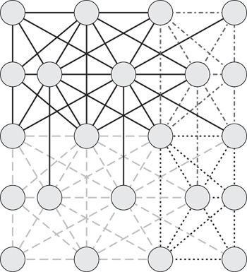
If, instead of coloring the graph by links where multiple links touch a single vertex and hence depend on each other, we color the graph in larger chunks, we reduce the number of colors we need. The number of neighboring chunks, and hence colors, touched by the links emanating from a given chunk will be reduced thanks to the lower density at which the coloring is applied. We can see an example of this chunking in Figure 17.10.3 Thanks to the coloring of the chunks themselves, we know that any two chunks of a given color and hence in a given batch are independent. The result of this is that each chunk within a given batch can be executed by a different OpenCL work-group with no further intergroup synchronization requirements.
Figure 17.10 Dividing the mesh into larger chunks and applying a coloring to those. Note that fewer colors are needed than in the direct link coloring approach. This pattern can repeat infinitely with the same four colors.
The benefit of reducing the number of colors is that we reduce the number of levels of global synchronization required. Each global synchronization in OpenCL requires a kernel dispatch and completion event; reducing the total number of dispatches significantly reduces the overhead of simulation.
These chunks of the graph are grown out from a single vertex in a breadth-first fashion. From a starting vertex we add all of the connected links and enqueue all of the vertices at the far ends of those links. From those vertices we perform the same addition of all connected links not already added and add their vertices to the queue. Eventually we build a chunk to our desired size. The size can be parameterized; 256 has been a good number in experiments.
Of course, while we have independent chunks within a batch, links within a chunk are still interdependent as in the naïve coloring. Within any given batch, represented by a single color of the graph, we perform a second level of coloring. This coloring is linkwise and identical in principle to the previously discussed single-level batching except that only links within a given batch need be considered. We can iterate through the local colors of links using an in-kernel for loop. Of course, depending on the size of each chunk, we may have more or fewer links in a given local batch than work-items in a group. We can rectify this by arranging the local batches so that there are more than what is absolutely necessary: rather than simply creating arbitrarily sized batches of links, we pack links into work-group-size batches and move on to another when either there is a dependence or a batch is full. Using this two-layer batching, we move to code like the following:
__kernel void
SolvePositionsFromLinksKernel(
const int startLink,
const int numLinks,
const float kst,
const float ti,
__global int2 * g_linksVertexIndices,
__global float * g_linksMassLSC,
__global float * g_linksRestLengthSquared,
__global float * g_verticesInverseMass,
__global float4 * g_vertexPositions)
{
for( batch = 0; batch < numLocalBatches; ++batch )
{
// Assume that links are sorted in memory in order of
// local batches within groups
int linkID = get_global_id(0)*batch;
float massLSC = g_linksMassLSC[linkID];
float restLengthSquared = g_linksRestLengthSquared[linkID];
if( massLSC > 0.0f ) {
int2 nodeIndices = g_linksVertexIndices[linkID];
int node0 = nodeIndices.x;
int node1 = nodeIndices.y;
float3 position0 = g_vertexPositions[node0].xyz;
float3 position1 = g_vertexPositions[node1].xyz;
float inverseMass0 = g_verticesInverseMass[node0];
float inverseMass1 = g_verticesInverseMass[node1];
float3 del = position1 - position0;
float len = dot(del, del);
float k = ((restLengthSquared –
len)/(massLSC*(restLengthSquared+len)))*kst;
position0 = position0 - del*(k*inverseMass0);
position1 = position1 + del*(k*inverseMass1);
g_vertexPositions[node0] = (float4)(position0, 0.f);
g_vertexPositions[node1] = (float4)(position1, 0.f);
}
barrier(CLK_GLOBAL_MEM_FENCE);
}
}
Note that to correctly satisfy OpenCL inter-work-item memory consistency we must include barrier instructions on each loop iteration. Of course, because they are in a loop, these barrier instructions must be executed by all work-items in the work-group; the batches should be created such that all work-items see the same number with no early exit from the loop. In reality we are unlikely to perfectly fill the batches; there will be SIMD lanes lying idle at various points in the computation (or writing data that will be ignored). This is unfortunate but unavoidable, and the efficiency savings from reducing global synchronization trade against this. Note that the solver algorithm hasn’t changed, only the pattern of link solving used to achieve it. This does mean that any given batching produces a subtly different output from all other batchings because of the ordering of floating-point operations; however, any given batching is deterministic.
Note as well that in this case we are still operating inefficiently in global memory. Given that within a group the links will reuse vertex data, and that vertex data will not be shared with other work-groups, we can cache the vertex data in OpenCL local memory. We will see final code that does this in the next section.
Optimizing for SIMD Computation and Local Memory
In the current generation high-end GPUs are all SIMD architectures. Current architectures from AMD and NVIDIA include up to 24 cores each with 16- or 32-wide SIMD units. Logical SIMD vectors can be wider: a 64-element vector is executed over four consecutive cycles on 16 SIMD lanes on the AMD Radeon HD 6970 architecture by replaying the same instruction four times.
These wide SIMD vectors give a certain level of guaranteed synchronization. We know that any instruction issued on the HD 6970 will be executed at the same time across 64 work-items, with no need for barrier synchronization. With the AMD compiler and runtime, barriers will be automatically converted to no-ops if the work-group size is the same as or smaller than the hardware vector size (known as a wavefront).
The consequence of this guaranteed synchronization is that if we define our work-groups appropriately and aim for batch sizes and data layouts that map efficiently to groups of vector-width work-items, we can generate efficient code that does not require barrier synchronization to execute correctly. Indeed, it is safe to drop the barriers entirely as long as we insert memory fences (mem_fence(CLK_GLOBAL_MEM_FENCE) or mem_fence(CLK_LOCAL_MEM_FENCE)) to ensure that the compiler does not reorder memory operations inappropriately.
As mentioned earlier, we can go one step further. Recall what we saw in the previous section:
for each batch of work-groups:
for each batch of links within the chunk:
process link
barrier;
Now let’s slightly change the algorithm:
for each batch of wavefronts:
load all vertex data needed by the chunk
for each batch of links within the wavefront
process link using vertices in local memory
local fence
store updated vertex data back to global memory
This saves on synchronization, and there is reuse of vertex data within efficient local memory, reducing the amount of global memory traffic and further improving performance. To achieve this we prepare a list of vertices to load as extra per-wavefront data and first scan this list to load vertices. We update the link data to contain local vertex indices rather than global vertex indices. When processing the links local batch by local batch within the chunk, the loaded link data indexes the local vertex buffer where the vertices are updated in place. After the chunk is complete, the vertices are written back to global memory.
Our final kernel, including loading from shared memory, using fences rather than barriers, and working on a wavefront basis, is seen here:
__kernel void
SolvePositionsFromLinksKernel(
const int startWaveInBatch,
const int numWaves,
const float kst,
const float ti,
__global int2 *g_wavefrontBatchCountsVertexCounts,
__global int *g_vertexAddressesPerWavefront,
__global int2 * g_linksVertexIndices,
__global float * g_linksMassLSC,
__global float * g_linksRestLengthSquared,
__global float * g_verticesInverseMass,
__global float4 * g_vertexPositions,
__local int2 *wavefrontBatchCountsVertexCounts,
__local float4 *vertexPositionSharedData,
__local float *vertexInverseMassSharedData)
{
const int laneInWavefront =
(get_global_id(0) & (WAVEFRONT_SIZE-1));
const int wavefront = startWaveInBatch + (get_global_id(0) /
WAVEFRONT_SIZE);
const int firstWavefrontInBlock = startWaveInBatch +
get_group_id(0) * WAVEFRONT_BLOCK_MULTIPLIER;
const int localWavefront = wavefront - firstWavefrontInBlock;
// Mask out in case there's a stray "wavefront" at the
// end that's been forced in through the multiplier
if( wavefront < (startWaveInBatch + numWaves) ) {
// Load the batch counts for the wavefronts
// Mask out in case there's a stray "wavefront"
// at the end that's been forced in through the multiplier
if( laneInWavefront == 0 ) {
int2 batchesAndVertexCountsWithinWavefront =
g_wavefrontBatchCountsVertexCounts[wavefront];
wavefrontBatchCountsVertexCounts[localWavefront] =
batchesAndVertexCountsWithinWavefront;
}
mem_fence(CLK_LOCAL_MEM_FENCE);
int2 batchesAndVerticesWithinWavefront =
wavefrontBatchCountsVertexCounts[localWavefront];
int batchesWithinWavefront =
batchesAndVerticesWithinWavefront.x;
int verticesUsedByWave = batchesAndVerticesWithinWavefront.y;
// Load the vertices for the wavefronts
for( int vertex = laneInWavefront;
vertex < verticesUsedByWave;
vertex+=WAVEFRONT_SIZE ) {
int vertexAddress = g_vertexAddressesPerWavefront[
wavefront*MAX_NUM_VERTICES_PER_WAVE + vertex];
vertexPositionSharedData[localWavefront*
MAX_NUM_VERTICES_PER_WAVE + vertex] =
g_vertexPositions[vertexAddress];
vertexInverseMassSharedData[localWavefront*
MAX_NUM_VERTICES_PER_WAVE + vertex] =
g_verticesInverseMass[vertexAddress];
}
mem_fence(CLK_LOCAL_MEM_FENCE);
// Loop through the batches performing the solve on each in LDS
int baseDataLocationForWave = WAVEFRONT_SIZE * wavefront *
MAX_BATCHES_PER_WAVE;
//for( int batch = 0; batch < batchesWithinWavefront; ++batch )
int batch = 0;
do {
int baseDataLocation =
baseDataLocationForWave + WAVEFRONT_SIZE * batch;
int locationOfValue = baseDataLocation + laneInWavefront;
// These loads should all be perfectly linear across the WF
int2 localVertexIndices =
g_linksVertexIndices[locationOfValue];
float massLSC = g_linksMassLSC[locationOfValue];
float restLengthSquared =
g_linksRestLengthSquared[locationOfValue];
// LDS vertex addresses based on logical wavefront
// number in block
// and loaded index
int vertexAddress0 = MAX_NUM_VERTICES_PER_WAVE *
localWavefront + localVertexIndices.x;
int vertexAddress1 =
MAX_NUM_VERTICES_PER_WAVE * localWavefront +
localVertexIndices.y;
float4 position0 = vertexPositionSharedData[vertexAddress0];
float4 position1 = vertexPositionSharedData[vertexAddress1];
float inverseMass0 =
vertexInverseMassSharedData[vertexAddress0];
float inverseMass1 =
vertexInverseMassSharedData[vertexAddress1];
float4 del = position1 - position0;
float len = mydot3(del, del);
float k = 0;
if( massLSC > 0.0f ) {
k = ((restLengthSquared - len)/
(massLSC*(restLengthSquared+len)))*kst;
}
position0 = position0 - del*(k*inverseMass0);
position1 = position1 + del*(k*inverseMass1);
// Ensure compiler does not reorder memory operations
mem_fence(CLK_LOCAL_MEM_FENCE);
vertexPositionSharedData[vertexAddress0] = position0;
vertexPositionSharedData[vertexAddress1] = position1;
// Ensure compiler does not reorder memory operations
mem_fence(CLK_LOCAL_MEM_FENCE);
++batch;
} while( batch < batchesWithinWavefront );
// Update the global memory vertices for the wavefronts
for( int vertex = laneInWavefront;
vertex < verticesUsedByWave;
vertex+=WAVEFRONT_SIZE ) {
int vertexAddress = g_vertexAddressesPerWavefront[wavefront*
MAX_NUM_VERTICES_PER_WAVE + vertex];
g_vertexPositions[vertexAddress] =
(float4)(vertexPositionSharedData[localWavefront*
MAX_NUM_VERTICES_PER_WAVE + vertex].xyz, 0.f);
}
}
}
What we have tried to demonstrate is that these architectures are not scalar architectures, and work-items are not independent, in architectural terms not threads. For efficiency, just as we have to optimize for SSE vectors on x86 hardware to attain full performance, for the GPU we can use the architectural features to improve performance of our algorithms. The warning in this is that our code is no longer portable across architectures. In the Bullet code we currently provide SIMD-optimized and portable versions of this solver.
Adding OpenGL Interoperation
The final subject we should discuss here is interoperation with OpenGL. This was discussed earlier in Chapter 10, and cloth simulation is a good example of where such interoperation is useful outside of image processing.
When we render soft-body objects on the screen, we create a render call and pass it a vertex buffer object, or VBO. This describes a memory buffer in GPU memory containing a list of all vertices that we need to draw. In addition, we provide buffers containing triangle index lists that reference the vertex buffer, and appropriate texture and normal buffers. If we render the output of the soft-body simulation, the vertex positions and normals are computed on each step of the simulation; the vertex and normal buffers used for rendering must be updated with these new values.
Updating these values via copying back to host memory, performing another copy into a structure to upload, and then uploading this to the vertex buffer adds additional overhead in terms of bus synchronization time and bandwidth. OpenCL/OpenGL interoperability reduces this problem. We can directly write using an OpenCL kernel into a buffer that will be used by the OpenGL rendering code. All data can stay in high-speed device memory with none of the overhead of copying back to the host and up to the GPU again.
On the host side we create a vertex struct with the necessary fields for rendering and create a buffer from this and a VBO handle:
struct vertex_struct
{
float pos[3];
float normal[3];
float texcoord[2];
};
vertex_struct* cpu_buffer = new . . .
GLuint clothVBO;
From these objects we create a device-side VBO with the GL_DYNAMIC_DRAW flag that specifies that this buffer will be updated on a regular basis:
// Construct VBO
glGenBuffers(1, &clothVBO);
glBindBuffer(GL_ARRAY_BUFFER, clothVBO);
// Do initial upload to ensure that the buffer exists on the device
// this is important to allow OpenCL to make use of the VBO
glBufferData(GL_ARRAY_BUFFER, sizeof(vertex_struct)*width*height,
&(cpu_buffer[0]), GL_DYNAMIC_DRAW);
glBindBuffer(GL_ARRAY_BUFFER, 0);
To render we use the VBO as a source for vertex data using the following code:
// Enable vertex, normal, and texture arrays for drawing
glBindBuffer(GL_ARRAY_BUFFER, clothVBO);
glEnableClientState(GL_VERTEX_ARRAY);
glEnableClientState(GL_NORMAL_ARRAY);
glEnableClientState(GL_TEXTURE_COORD_ARRAY);
glBindTexture(GL_TEXTURE_2D, texture);
// Set up vertex buffer state and draw
glVertexPointer(
3,
GL_FLOAT,
sizeof(vertex_struct),
(const GLvoid *)0 );
glNormalPointer(
GL_FLOAT,
sizeof(vertex_struct),
(const GLvoid *)(sizeof(float)*3) );
glTexCoordPointer(
2,
GL_FLOAT,
sizeof(vertex_struct),
(const GLvoid *)(sizeof(float)*6) );
glDrawElements(
GL_TRIANGLES,
(height-1 )*(width-1)*3*2,
GL_UNSIGNED_INT,
indices);
// Clean up code
glDisableClientState(GL_NORMAL_ARRAY);
glDisableClientState(GL_VERTEX_ARRAY);
glDisableClientState(GL_TEXTURE_COORD_ARRAY);
glBindTexture(GL_TEXTURE_2D, 0);
glBindBuffer(GL_ARRAY_BUFFER, 0);
The OpenCL code will first, at some point during setup, create a CL buffer from the GL buffer (it is for this reason that the GL buffer must be initialized with data). Then on each frame, after the OpenCL kernels have output the result of a time step of the simulation, the OpenCL version of the OpenGL buffer is acquired for use by OpenCL and can be used as a target by a kernel. Subsequently the buffer is freed and ready to be used again by OpenGL for rendering:
clBuffer = clCreateFromGLBuffer(
m_context,
CL_MEM_WRITE_ONLY,
clothVBO,
&ciErrNum);
clEnqueueAcquireGLObjects(m_cqCommandQue, 1, &clBuffer, 0, 0, NULL);
clEnqueueReleaseGLObjects(m_cqCommandQue, 1, &clBuffer, 0, 0, 0);
In this fashion we efficiently generate vertex data for rendering by an OpenGL application using the OpenCL soft-body simulation.