Chapter 16. Parallelizing Dijkstra’s Single-Source Shortest-Path Graph Algorithm
By Dan Ginsburg, P. Ellen Grant, and Rudolph Pienaar
FreeSurfer is a neuroimaging tool developed by the Martinos Center for Biomedical Imaging at Massachusetts General Hospital. The tool is capable of creating triangular-mesh structural reconstructions of the cortical surface of the brain from MRI images. As part of a research study into the curvature of the cortical surface of the human brain, a set of curvature measures was stored at each edge of this mesh.1 In order to assess the quality of the curvature measures and understand the underlying curvature of the brain surface, it was necessary to search along the mesh to find the shortest curvature values from various starting points on the brain to all other vertices along the rest of the surface. The performance of the existing Dijkstra’s algorithm on the CPU was proving too slow and making it difficult to study this curvature across many subjects and curvature measurement types. As a consequence, we created an OpenCL-based parallel implementation of Dijkstra’s algorithm.
This chapter presents this implementation of Dijkstra’s algorithm using OpenCL, which can leverage any of the available compute hardware on the host based on the algorithm in “Accelerating Large Graph Algorithms on the GPU Using CUDA” by Pawan Harish and P. J. Narayanan.2 It covers how to map the graph into data structures that can be easily accessed by parallel hardware and describes the implementation of the kernels that compute Dijkstra’s algorithm in parallel. Finally, it covers the details of how to partition the workload to run on multiple compute devices. Our implementation of Dijkstra’s algorithm is provided in the Chapter_16/Dijkstra directory of the book’s source code examples.
Graph Data Structures
The first step in getting Dijkstra’s algorithm onto the GPU is to create a graph data structure that is efficiently accessible by the GPU. The graph is composed of vertices and edges that connect vertices together. Each edge has a weight value associated with it that typically measures some cost in traveling across that edge. In our case, the edge weights were determined by the curvature function as we were interested in minimizing curvature values in traveling across the mesh. In a mapping application, the edge weights would usually be the physical distance between nodes. The data structures used in our implementation are the same as those described in “Accelerating Large Graph Algorithms on the GPU Using CUDA.” The graph is represented as a collection of arrays:
• int *vertexArray: Each entry contains an index into the first element of edgeArray to be used as an edge for that vertex. The edges are stored sequentially in the edge array, and the number of edges for vertexArray[N] is the sequence of vertices up to the index stored in vertexArray[N+1] (or the size of edgeArray if N is the last element of vertexArray).
• int *edgeArray: Each element is an index to the vertex that is connected by edge to the current vertex. Note that edges are assumed to be one-directional from the source to the destination vertex. For edges that are bidirectional, an entry must be placed in the table for each direction.
• int *weightArray: For each edge in edgeArray, this array stores the weight value of the edge. There is one weight value for each edge.
These three arrays form the totality of graph data that an application needs to set up in order to run Dijkstra’s algorithm using our implementation. The implementation itself requires three more arrays that are used by the kernels during the computation:
• int *maskArray: This array stores a value of 0 or 1 for each vertex, which determines whether the algorithm needs to continue processing for that node. The reason integer type was chosen over a byte representation is that certain implementations of OpenCL do not support accessing byte-aligned arrays.
• float *updatingCostArray: This is a buffer used during the algorithm to store the current cost computed to the vertex.
• float *costArray: This stores the final computed minimum cost for each vertex.
The only other piece of information the algorithm needs is which source vertices to run the algorithm for and a host-allocated array to store the results. Each execution of Dijkstra will output an array the size of the number of vertices in the graph with the total cost of the shortest distance from the source vertex to each vertex in the graph. An example of the C structure and function used to execute Dijkstra’s algorithm using OpenCL on a single GPU is provided in Listing 16.1.
Listing 16.1 Data Structure and Interface for Dijkstra’s Algorithm
typedef struct
{
// (V) This contains a pointer to the edge list for each vertex
int *vertexArray;
// Vertex count
int vertexCount;
// (E) This contains pointers to the vertices that each edge
// is attached to
int *edgeArray;
// Edge count
int edgeCount;
// (W) Weight array
float *weightArray;
} GraphData;
/// Run Dijkstra's shortest path on the GraphData provided to this
/// function. This function will compute the shortest-path distance
/// from sourceVertices[n] -> endVertices[n] and store the cost in
/// outResultCosts[n]. The number of results it will compute is
/// given by numResults.
///
/// This function will run the algorithm on a single GPU.
///
/// param gpuContext Current GPU context, must be created by
/// caller
/// param deviceId The device ID on which to run the kernel.
/// This can be determined externally by the
/// caller or the multi-GPU version will
/// automatically split the work across
/// devices
/// param graph Structure containing the vertex, edge, and
/// weight array for the input graph
/// param startVertices Indices into the vertex array from
/// which to start the search
/// param outResultsCosts A pre-allocated array where the
/// results for each shortest-path
/// search will be written. This
/// must be sized numResults *
/// graph->numVertices.
/// param numResults Should be the size of all three passed
/// in arrays
void runDijkstra( cl_context gpuContext, cl_device_id deviceId,
GraphData* graph,
int *sourceVertices, float *outResultCosts,
int numResults );
Kernels
The high-level loop that executes the algorithm using OpenCL is provided in pseudo code in Listing 16.2.
Listing 16.2 Pseudo Code for High-Level Loop That Executes Dijkstra’s Algorithm
foreach sourceVertex to search from
// Initialize all of maskArray[] to 0
// Initialize all of costArray[] to MAX
// Initialize all of updatingCostArray[] to MAX
// Initialize maskArray[sourceVertex] to 1
// Initialize costArray[sourceVertex],
// updatingCostArray[sourceVertex] to 0
initializeMaskAndCostArraysKernel()
// While any element of maskArray[] != 0
while ( ! maskArrayEmpty() )
// Enqueue phase 1 of the Dijkstra kernel for all vertices
enqueueKernelPhase1()
// Enqueue phase 2 of the Dijkstra kernel for all vertices
enqueueKernelPhase2()
// Read the mask array back from the device
readMaskArrayFromDeviceToHost()
// Read final cost array for sourceVertex to the device and
// store it on the host
readCostArrayFromDeviceToHost()
The first kernel that is queued to OpenCL for each source vertex is simply responsible for initialization of buffers. This was done using a kernel rather than on the CPU to reduce the amount of data transferred between the CPU and GPU. The initialization kernel is provided in Listing 16.3 and is executed during the initializeMaskAndCostArraysKernel() from the pseudo code in Listing 16.2.
Listing 16.3 Kernel to Initialize Buffers before Each Run of Dijkstra’s Algorithm
__kernel void initializeBuffers( __global int *maskArray, __global
float *costArray,
__global float *updatingCostArray,
int sourceVertex, int vertexCount )
{
int tid = get_global_id(0);
if (sourceVertex == tid)
{
maskArray[tid] = 1;
costArray[tid] = 0.0;
updatingCostArray[tid] = 0.0;
}
else
{
maskArray[tid] = 0;
costArray[tid] = FLT_MAX;
updatingCostArray[tid] = FLT_MAX;
}
}
The algorithm itself is broken into two phases. This is necessary because there is no synchronization possible outside of local work-groups in OpenCL, and this would be required to execute the kernel algorithm in a single phase. The first phase of the algorithm visits all vertices that have been marked in the maskArray and determines the cost to each neighbor. If the current cost plus the new edge weight is less than what is currently stored in updatingCostArray, then that new cost is stored for the vertex. The second phase of the algorithm checks to see if a smaller cost has been found for each vertex and, if so, marks it as needing visitation and updates the costArray. At the end of kernel phase 2, the updatingCostArray is synchronized with the costArray. The two phases of the algorithm are provided in Listing 16.4.
Listing 16.4 Two Kernel Phases That Compute Dijkstra’s Algorithm
__kernel void DijkstraKernel1(__global int *vertexArray,
__global int *edgeArray,
__global float *weightArray,
__global int *maskArray,
__global float *costArray,
__global float *updatingCostArray,
int vertexCount, int edgeCount )
{
int tid = get_global_id(0);
if ( maskArray[tid] != 0 )
{
maskArray[tid] = 0;
int edgeStart = vertexArray[tid];
int edgeEnd;
if (tid + 1 < (vertexCount))
{
edgeEnd = vertexArray[tid + 1];
}
else
{
edgeEnd = edgeCount;
}
for(int edge = edgeStart; edge < edgeEnd; edge++)
{
int nid = edgeArray[edge];
if (updatingCostArray[nid] > (costArray[tid] +
weightArray[edge]))
{
updatingCostArray[nid] = (costArray[tid] +
weightArray[edge]);
}
}
}
}
__kernel void DijkstraKernel2(__global int *vertexArray,
__global int *edgeArray,
__global float *weightArray,
__global int *maskArray,
__global float *costArray,
__global float *updatingCostArray,
int vertexCount)
{
// access thread id
int tid = get_global_id(0);
if (costArray[tid] > updatingCostArray[tid])
{
costArray[tid] = updatingCostArray[tid];
maskArray[tid] = 1;
}
updatingCostArray[tid] = costArray[tid];
}
Leveraging Multiple Compute Devices
In order to leverage multiple compute devices, the workload needs to be partitioned. The approach taken in our implementation is to partition the number of searches across the available compute hardware. The application detects the number of GPU and CPU devices and splits the workload across the devices. The way the vertices are allocated to threads is by dynamically determining a work size based on the result of querying OpenCL for the value of GL_DEVICE_MAX_WORKGROUP_SIZE.
As can be seen in Listing 16.4, each of the kernels is written to process one vertex at a time. The implementation sets the OpenCL local work size to the value of querying GL_DEVICE_MAX_WORKGROUP_SIZE for the device. The global work-group size is equal to the vertex count rounded up to the closest maximum work-group size. The maskArray, costArray, and updatingCostArray are padded to this size so that the kernels do not need to check whether thread IDs are outside the bounds of the array. This workload portioning essentially means that each thread on the device will process a single vertex. In the case of a CPU device, the OpenCL implementation will multithread the implementation across the available cores.
In the case of mixing multiple devices, each device is allocated its own CPU thread for communicating with OpenCL. The reason this is done in multiple threads rather than a single thread is that the algorithm requires reads back from host to device on each iteration of the inner loop of the algorithm (Listing 16.2). In general, a more favorable approach would be to queue all of the kernel executions from a single thread to all devices. One additional consideration is that typically there is a performance difference between the ability of the CPU and GPU to process kernels. As such, rather than choosing a fixed allocation of searches to each device, a future extension would be to examine OpenCL performance-related queries (or run a dynamic benchmark at start-up) and allocate the searches across the devices based on some performance characteristics. This would likely yield better performance as the current implementation must wait until the slowest device finishes execution.
The implementation of Dijkstra’s algorithm was tested on an x86_64 Linux PC with an Intel Core i7 960 CPU @ 3.20GHz with an NVIDIA GTX 295 GPU running the NVIDIA 260.19.21 driver. In summary, the performance speedup using the GPU was dependent on the size of the graph (number of vertices) and the degree of the graph (number of edges per vertex). As the number of vertices in the graph increases, the GPU tends to outperform the CPU by a wider margin. In the best case measured, the dual-GPU implementation was 11.1 times faster than the CPU implementation.
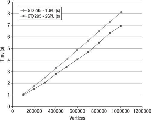
The data in Table 16.1 was collected from randomly generated graphs containing a degree (edges per vertex) of 5. These graphs were run through the OpenCL-based GPU and multi-GPU implementations of Dijkstra’s algorithm selecting 100 starting vertices. Additionally, the data sets were run through a single-threaded CPU reference implementation of Dijkstra’s algorithm. The timings for each run are provided in seconds, and the data is summarized in Figures 16.1 and 16.2.
Table 16.1 Comparison of Data at Vertex Degree 5
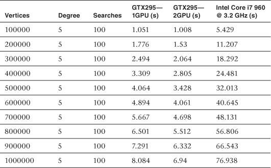
Figure 16.1 Summary of data in Table 16.1: NV GTX 295 (1 GPU, 2 GPU) and Intel Core i7 performance
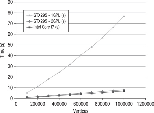
Figure 16.2 Using one GPU versus two GPUs: NV GTX 295 (1 GPU, 2 GPU) and Intel Core i7 performance
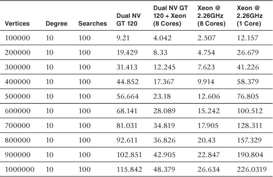
The data in Table 16.2 was collected using the same test setup as for Table 16.1; the only difference was that the degree of the graph was set at 10 instead of 5. Increasing the degree of the graph reduced the advantage of the GPU implementation over the CPU (from 9.18 times on average down to 6.89 times), but the GPU version still has a significant advantage. The results from Table 16.2 are shown in Figure 16.3.
Table 16.2 Comparison of Data at Vertex Degree 10
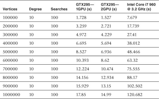
Figure 16.3 Summary of data in Table 16.2: NV GTX 295 (1 GPU, 2 GPU) and Intel Core i7 performance—10 edges per vertex
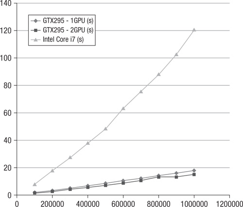
As can be seen from the collected performance data, regardless of the number of edges, the performance advantage the GPU implementation has over the CPU in terms of absolute seconds grows with the size of the graph. The setup costs associated with transferring data to the GPU and submitting/waiting for the kernels are better masked the more data is present. Some amount of GPU-to-CPU communication is necessary because the algorithm is by nature dynamic and the runtime length and iterations are not known before execution of the algorithm.
The only platform available to us to test the hybrid CPU-GPU implementation of Dijkstra was a MacPro with dual Quad-Core Intel Xeon CPUs @ 2.26GHz and dual NVIDIA GeForce GT 120 GPUs (note that these are rather low-end GPUs with only four compute units). The testing compared running on a single core of the CPU, running on all eight cores of the CPU using OpenCL, running on both GPUs, and combining both GPUs with the use of all eight CPU cores.
The performance results are detailed in Table 16.3 and Figure 16.4. In all tests, the best performance was attained by running the multicore CPU-only version using OpenCL. The next-best performance was combining the Dual NV GT 120 GPUs and the multicore CPU. It was initally rather surprising that the dual GPU+CPU implementation was bested by the CPU-only version. However, this was likely because the GPUs have only four compute units and the algorithm has a lot of CPU/GPU traffic. As such, the cost of switching threads and CPU/GPU communication offset the gains of running purely on the CPU.
Figure 16.4 Summary of data in Table 16.3: comparison of dual GPU, dual GPU + multicore CPU, multicore CPU, and CPU at vertex degree 1
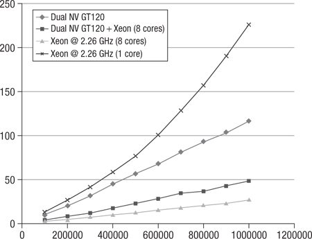
Beyond that, the results were as expected: the reference single-core CPU performance fared the poorest and the Dual NV GT 120 GPU lagged behind combining the Dual NV GT 120 GPU + multicore CPU. Because Dijkstra’s algorithm requires a significant number of calls to the OpenCL runtime and high traffic between the CPU and GPU, the performance gain was not as significant as one would expect from a different algorithm that requires less overhead between the host and device. However, the approach taken in the sample code should provide a useful example for how in general one can combine multiple GPUs and the CPU using OpenCL.
Table 16.3 Comparison of Dual GPU, Dual GPU + Multicore CPU, Multicore CPU, and CPU at Vertex Degree 10