Chapter 19. Optical Flow
Optical flow is a fundamental concept in computer vision. Optical flow describes the motion that occurs between images and has application in image stabilization, frame rate upsampling, and motion or gesture analysis. In this chapter, we will discuss an implementation of pyramidal Lucas-Kanade (LK) optical flow.1 Sub-pixel accuracy is essential to the implementation and is maintained by a number of resampling operations requiring linear interpolation. As we will see, the texture-filtering hardware on the GPU can be used to perform linear interpolation of data, which can provide significant speedups. Additionally, we will discuss how local memory and early kernel exit techniques provide acceleration.
Optical Flow Problem Overview
Optical flow describes the motion that occurs between images. At each point in the image, we will compute a 2D flow vector that describes the motion that occurred between points in the images. This is called “dense” optical flow because it produces a dense set of vectors for the entire image, in contrast to tracking only a few sparse points. Optical flow is computationally intensive, and other implementations attempt only sparse computation, whereas we will discuss a dense implementation that achieves high performance on a GPU using OpenCL.
As an intuitive explanation, consider the situation where we know the gradient of the image at some location. This tells us if it is getting brighter or darker in some direction. If we later observe that the location itself has become brighter or darker, we can make some inference as to the motion of the image content. This makes the assumption that the brightness of the object itself isn’t changing and so the change in pixel brightness is due to motion. Given two images I(x, y) and J(x, y), we seek to find the image velocities dx and dy that minimize the residual error:
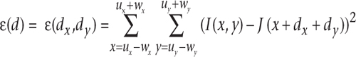
Here we have a window of size (wx, wy) centered around a point (ux, uy), where (x, y) denotes the position in the window. Thus for each pixel with its surrounding window, we are searching for the motion that minimizes the difference in brightness, indicating where that region has moved.
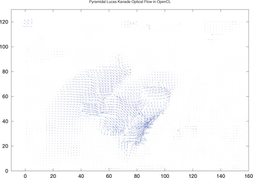
This chapter presents an implementation of optical flow using OpenCL. In the discussion, we will use test images from the “MiniCooper”2 data set. Figure 19.1 shows two images from this set where we see that a man is closing the trunk of a car. Figure 19.2 shows the recovered motion vectors from two sequential images in the set. The motion vectors occur around the area of the trunk and where the man moves; both areas have vectors generally pointing downward as the trunk closes.
Figure 19.1 A pair of test images of a car trunk being closed. The first (a) and fifth (b) images of the test sequence are shown.
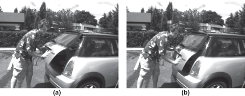
Figure 19.2 Optical flow vectors recovered from the test images of a car trunk being closed. The fourth and fifth images in the sequence were used to generate this result.
There are many methods of finding the optical flow between images. Here we discuss the implementation of pyramidal Lucas-Kanade optical flow, which is presented because it is a widely known and studied algorithm that may be familiar to the reader and facilitates discussion of the GPU mappings.
Computationally, Lucas-Kanade optical flow minimizes the residual error, which reduces essentially to finding the optical flow v = [vx, vy]T as
![]()
The matrix G and vector b are given by the image values I, J and derivatives Ix, Iy, and Ixy (the product of Ix and Iy):
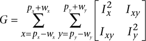
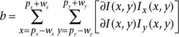
Here ∂I(x, y) is termed the image difference and b the mismatch vector.
The algorithm operates on image pyramids. Each level of the image pyramid is the same image with different scales. The bottom of the pyramid is the initial image, and each pyramid level is the image scaled by some scaling factor. In our implementation each level is scaled by 0.5 in each image dimension.
The image difference at level L for iteration k is computed as
![]()
Pyramidal Lucas-Kanade optical flow is an iterative scheme, where equation (2) is evaluated iteratively at each position for k iterations, with the guess for the flow vector being refined (x′, y′) = (x + vx, y + vy) at each iteration, at each level. Here, (gLx, gLy) is the guess for the flow from the previous pyramid level, and (vkx, vky) is the calculation of the flow at iteration k at the present level. The iterative reevaluation of equation (2) requires heavy computation.
The algorithm proceeds from the upper levels L down to level 0 (full-size image).
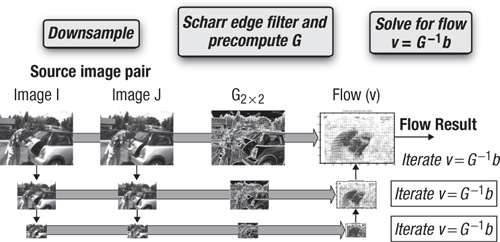
At each level, the flow vector, v = [vx, vy]T, computed from the previous level is used as a starting guess to the current level, and for the initial level it is initialized as (0, 0). Figure 19.3 depicts an implementation of the pyramidal LK optical flow algorithm based on the image pyramid structure. It shows the process of downsampling the images, computing image derivatives and the matrix G, and then computing the flow from smallest to largest pyramid level.
Figure 19.3 Pyramidal Lucas-Kanade optical flow algorithm
First, we discuss the overall approach to mapping this to the GPU. The algorithm begins by creating the image pyramids, storing each level in texture memory on the GPU. From the equations, it can be seen that we need image pyramids for the images, I, J, and derivatives, Ix, Iy. Image pyramid creation proceeds from the base pyramid level and generates successively high levels. For each pyramid level, images are filtered in two kernels that implement a separable filter. A separable filter implements a 2D filter kernel as two 1D filter kernel passes. In our implementation we implement a 5×5 filter kernel by horizontal 1×5 and vertical 5×1 filter kernels. These kernels simply read image values around a center pixel and calculate a weighted sum. The horizontal kernel can be implemented as shown in the next code block. Note that we have omitted code to perform efficient coalesced memory writes and use textures for simplicity and because the majority of the time is spent computing the flow kernel shown later.
__kernel void downfilter_x_g(
__read_only image2d_t src,
__global uchar *dst, int dst_w, int dst_h )
{
sampler_t srcSampler = CLK_NORMALIZED_COORDS_FALSE |
CLK_ADDRESS_CLAMP_TO_EDGE |
CLK_FILTER_NEAREST ;
const int ix = get_global_id(0);
const int iy = get_global_id(1);
float x0 =
read_imageui( src, srcSampler, (int2)(ix-2,iy)).x/16.0f;
float x1 =
read_imageui( src, srcSampler, (int2)(ix-1,iy)).x/4.0f;
float x2 =
(3*read_imageui( src, srcSampler, (int2)(ix,iy)).x)/8.0f;
float x3 =
read_imageui( src, srcSampler, (int2)(ix+1,iy)).x/4.0f;
float x4 =
read_imageui( src, srcSampler, (int2)(ix+2,iy)).x/16.0f;
int output = round( x0 + x1 + x2 + x3 + x4 );
if( ix < dst_w && iy < dst_h ) {
// uncoalesced when writing to memory object
// acceptable if caches present, otherwise should be written
// for coalesced memory accesses
dst[iy*dst_w + ix ] = (uchar)output;
}
}
Because we are downsampling, a lowpass filter is used and a decimation by two is also applied after filtering to create the next-higher (smaller) pyramid level. Note that we can avoid having a kernel only performing decimation. Instead, we can combine the decimation with the second, vertical filter pass by only performing the vertical pass at pixel locations that write to the next level after decimation. This can be done by launching a kernel that covers the dimensions of the upper level and multiplying the lookups by 2 to index into the lower level correctly before writing the results. The following code shows the vertical filtering and decimation kernel:
__kernel void downfilter_y_g(
__read_only image2d_t src,
__global uchar *dst, int dst_w, int dst_h )
{
sampler_t srcSampler = CLK_NORMALIZED_COORDS_FALSE |
CLK_ADDRESS_CLAMP_TO_EDGE |
CLK_FILTER_NEAREST ;
const int ix = get_global_id(0);
const int iy = get_global_id(1);
float x0 = read_imageui( src, srcSampler,
(int2)(2*ix,2*iy-2) ).x/16.0f;
float x1 = read_imageui( src, srcSampler,
(int2)(2*ix,2*iy-1) ).x/4.0f;
float x2 = (3*read_imageui( src, srcSampler,
(int2)(2*ix,2*iy) ).x)/8.0f;
float x3 = read_imageui( src, srcSampler,
(int2)(2*ix,2*iy+1) ).x/4.0f;
float x4 = read_imageui( src, srcSampler,
(int2)(2*ix,2*iy+2) ).x/16.0f;
int output = round(x0 + x1 + x2 + x3 + x4);
if( ix < dst_w-2 && iy < dst_h-2 ) {
dst[iy*dst_w + ix ] = (uchar)output;
}
}
Noting again the components of equations (3) and (4), we see that in addition to the image pyramid values, we require derivative values at each level of the pyramid. This is done by sending the newly computed image pyramid to kernels that compute the derivatives at each level. Note also that the derivative computation at each image level is independent of the others, and when supported, GPU hardware can run different derivative kernels concurrently for more efficiency. The derivative computation is a 3×3 filter kernel implemented in two passes as a separable filter.
Given the image pyramids for I and J and image derivative pyramids for each level of I, the flow is calculated according to equation (2), starting from the upper level of the pyramid, and propagating results down through pyramid levels until the base level is reached, generating dense optical flow results. The kernel for computing optical flow at each pyramid level is iterative, performing the computation a number of times. First note that for equation (2), the components v and b change each iteration. v is solved each iteration and so changes, and b has the following components, as shown in equation (5), which change each iteration:
![]()
The matrix G, however, remains fixed in position and its values remain the same and so can be precomputed at each image location and simply retrieved when needed at the first iteration of each computation of equation (2). Because G is composed of local sums of derivative values, each work-item reads the local x and y derivative values and computes a four-component image value. The four-component vector type serves in this case as a handy data type for storing the 2×2 matrix G. Depending on the accuracy required, G can be saved as an int4 data type, because for input pixels in the range of [0, 255] the maximum squared image derivative falls within the capabilities of a 32-bit integer. If the filters used for downsampling and derivatives produced only integer results, this maintains accuracy. In case more accuracy is desired, floating-point could be used throughout at the cost of increased memory access time and space requirements. The following kernel gathers the data for G into a single memory buffer. Here, FRAD is defined as the radius of the window within which G is gathered.
#define FRAD 4
// G is int4 output
// This kernel generates the "G" matrix
// (2x2 covariance matrix on the derivatives)
// Each thread does one pixel,
// sampling its neighborhood of +/- FRAD
// radius and generates the G matrix entries.
__kernel void filter_G( __read_only image2d_t Ix,
__read_only image2d_t Iy,
__global int4 *G, int dst_w, int dst_h )
{
sampler_t srcSampler = CLK_NORMALIZED_COORDS_FALSE |
CLK_ADDRESS_CLAMP_TO_EDGE |
CLK_FILTER_NEAREST ;
const int idx = get_global_id(0);
const int idy = get_global_id(1);
int Ix2 = 0;
int IxIy = 0;
int Iy2 = 0;
for( int j=-FRAD ; j <= FRAD; j++ ) {
for( int i=-FRAD ; i<= FRAD ; i++ ) {
int ix = read_imagei(Ix,srcSampler,(int2)(idx+i,idy+j)).x;
int iy = read_imagei(Iy,srcSampler,(int2)(idx+i,idy+j)).x;
Ix2 += ix*ix;
Iy2 += iy*iy;
IxIy += ix*iy;
}
}
int4 G2x2 = (int4)( Ix2, IxIy, IxIy, Iy2 );
if( idx < dst_w && idy < dst_h ) {
G[ idy * dst_w + idx ] = G2x2;
}
}
Now, with G, I, and J pyramids and the derivative pyramids calculated, the flow computation of equation (2) can be calculated in a single kernel. We now look at parts of a kernel that solves for the flow vector given G, I, and J pyramids and the derivative pyramids. This kernel iteratively solves the equation until some convergence criteria or maximum number of iterations is reached.
The following code shows the kernel solving for the optical flow. Some discussion of the kernel is presented inline. Note that I, Ix, and Iy are reading from local memory; those lines are omitted here and discussed later. Additionally, we are using a bilinear sampling object, bilinSampler, also discussed later. For now the inline discussion will focus on steps that compute the flow vector. We begin by showing the beginning of the kernel called lkflow, including its parameter and variable declarations, and computation of its indices for accessing the input images:
#define FRAD 4
#define eps 0.0000001f;
// NB: It's important that these match the launch parameters!
#define LOCAL_X 16
#define LOCAL_Y 8
__kernel void lkflow(
__read_only image2d_t I,
__read_only image2d_t Ix,
__read_only image2d_t Iy,
__read_only image2d_t G,
__read_only image2d_t J_float,
__global float2 *guess_in,
int guess_in_w,
__global float2 *guess_out,
int guess_out_w,
int guess_out_h,
int use_guess )
{
// declare some shared memory (see details below)
__local int smem[2*FRAD + LOCAL_Y][2*FRAD + LOCAL_X] ;
__local int smemIy[2*FRAD + LOCAL_Y][2*FRAD + LOCAL_X] ;
__local int smemI[2*FRAD + LOCAL_Y][2*FRAD + LOCAL_X] ;
// Create sampler objects. One is for nearest neighbor,
// the other for bilinear interpolation
sampler_t bilinSampler = CLK_NORMALIZED_COORDS_FALSE |
CLK_ADDRESS_CLAMP_TO_EDGE |
CLK_FILTER_LINEAR ;
sampler_t nnSampler = CLK_NORMALIZED_COORDS_FALSE |
CLK_ADDRESS_CLAMP_TO_EDGE |
CLK_FILTER_NEAREST ;
// Image indices. Note for the texture, we offset by 0.5 to
//use the center of the texel.
int2 iIidx = { get_global_id(0), get_global_id(1)};
float2 Iidx = { get_global_id(0)+0.5, get_global_id(1)+0.5 };
The next steps of the kernel shown here copy data into local memory, but the code and discussion are deferred until later:
// load some data into local memory because it will be reused
// frequently
// ( see details below )
// ...
Between levels, the motion estimated, n, is propagated as the starting input for the next level, appropriately scaled to account for the larger image size. The following code determines the appropriate lookup for the guess from the previous pyramid level, when available, and then retrieves and scales it:
float2 g = {0,0};
// Previous pyramid levels provide input guess. Use if available.
if( use_guess != 0 ) {
// lookup in higher level, div by two to find position
// because it's smaller
int gin_x = iIidx.x/2;
int gin_y = iIidx.y/2;
float2 g_in = guess_in[gin_y * guess_in_w + gin_x ];
// multiply the motion by two because we are in a larger level.
g.x = g_in.x*2;
g.y = g_in.y*2;
}
Next, G is read from its four-component data type buffer. It is then inverted to form a 2×2 matrix G-1. When inverting, a determinant is computed and care is taken to set the determinant to a small non-zero value in case of a 0 determinant because it is used as a divisor in the 2×2 matrix inversion. The following code shows the lookup of the G matrix values and the matrix inversion:
// invert G, 2x2 matrix, use float since
// int32 will overflow quickly
int4 Gmat = read_imagei( G, nnSampler, iIidx );
float det_G =
(float)Gmat.s0 * (float)Gmat.s3 -
(float)Gmat.s1 * (float)Gmat.s2 ;
// avoid possible 0 in denominator
if( det_G == 0.0f ) det_G = eps;
float4 Ginv = {
Gmat.s3/det_G, -Gmat.s1/det_G,
-Gmat.s2/det_G, Gmat.s0/det_G };
The kernel then proceeds by calculating the mismatch vector ∂Ik(x, y) in equation (5) to find b. Given G-1 and b, the updated motion is found as v = G−1b, and the process repeats until convergence or some maximum number of iterations. We can define convergence in this case as happening when the change in the motion vector is negligible, because in that case, the next iteration will look up similar values and the motion will remain negligible, indicating some local solution has been reached. The following code shows this iterative computation of the motion as well as the check for convergence:
// for large motions we can approximate them faster by applying
// gain to the motion
float2 v = {0,0};
float gain = 4;
for( int k=0 ; k < 8 ; k++ ) {
float2 Jidx = { Iidx.x + g.x + v.x, Iidx.y + g.y + v.y };
float2 b = {0,0};
float2 n = {0,0};
// calculate the mismatch vector
for( int j=-FRAD ; j <= FRAD ; j++ ) {
for( int i=-FRAD ; i<= FRAD ; i++ ) {
int Isample = smemI[tIdx.y + FRAD +j][tIdx.x + FRAD+ i];
float Jsample = read_imagef( J_float,bilinSampler,
Jidx+(float2)(i,j) ).x;
float dIk = (float)Isample - Jsample;
int ix,iy;
ix = smem[tIdx.y + FRAD +j][tIdx.x + FRAD+ i];
iy = smemIy[tIdx.y + FRAD +j][tIdx.x + FRAD+ i];
b += (float2)( dIk*ix*gain, dIk*iy*gain );
}
}
// Optical flow (Lucas-Kanade).
// Solve n = G^-1 * b
//compute n (update), mult Ginv matrix by vector b
n = (float2)(Ginv.s0*b.s0 + Ginv.s1*b.s1,Ginv.s2*b.s0
+ Ginv.s3*b.s1);
//if the determinant is not plausible,
//suppress motion at this pixel
if( fabs(det_G)<1000) n = (float2)(0,0);
// break if no motion
if( length(n) < 0.004 ) break;
// guess for next iteration: v_new = v_current + n
v = v + n;
}
int2 outCoords = { get_global_id(0), get_global_id(1) };
if( Iidx.x < guess_out_w && Iidx.y < guess_out_h ) {
guess_out[ outCoords.y * guess_out_w + outCoords.x ] =
(float2)(v.x + g.x, v.y + g.y);
}
} // end kernel
Sub-Pixel Accuracy with Hardware Linear Interpolation
Many algorithms require sub-pixel image sampling. In the case of our LK optical flow example, sub-pixel accuracy is required for computing the image difference of equation (5) at each iteration k and level L because after each iteration, the currently computed motion is used to resample the original image data by applying the following offset to the lookup:
![]()
This can be easily achieved by sending the current lookup location as floating-point values to a texture sampler function, with the sampler set to perform linear interpolation:
![]()
The GPU will return a bilinearly interpolated sample at the given location. Care should be taken when using linear interpolation to offset the texture coordinates by 0.5 appropriately, because typically the work-item and work-group IDs are used to create an integer index that then needs to be offset by 0.5 (the “center” of the texel) before applying any additional offsets, such as the motion vectors in our example. On NVIDIA GPUs, the CUDA programming guide contains full details on the interpolation performed by the hardware. Using hardware interpolation performs what would otherwise be four lookups and arithmetic operations in a single lookup.
Application of the Texture Cache
A useful feature of the texturing hardware on the GPU is the presence of a texture cache. The cache is useful when many samples are taken from a 2D spatially local area. This occurs frequently in many image-processing algorithms. In the case of our optical flow example, the iterative computation of the mismatch vector in equation (5) requires a number of 2D texture lookups within the window area (wx, wy), Additionally, note that the center of the window (px, py) varies, dependent on the current motion vector guess, and thus the window location varies per iteration and at each location because different areas of the image will exhibit different motions.
Despite the variations, the motions typically exhibit some degree of locality per iteration, the update will typically be small and sub-pixel, the motion will vary slowly across the image, and regions of an image will exhibit similar motions. The texture hardware caching mechanisms are transparent to the programmer, and no explicit code or limitations on the motion are imposed by the caching mechanism.
Using Local Memory
While the texture cache is useful, a programmer may wish to use it for all of I, J and derivative data Ix and Iy. On a GTX 460 graphics card, it was observed to achieve only about 65 percent cache hits (a runtime profiler, such as the CUDA Visual Profiler, can be used to retrieve these statistics for a kernel). Because so many textures are used, cache data may be evicted even though it may need to be reloaded later.
One observation is that for a given work-group, at each iteration of the flow, the same data for I, Ix, and Iy is repeatedly read from the texture. To alleviate the demands on the texture cache, we can use OpenCL local memory as a user-managed cache. Local memory (also referred to as shared memory in the terminology of CUDA hardware) is memory that resides at the processing units of a GPU and so can be accessed fast. For each work-group, we read from a tile of data the size of the work-group plus a border whose width is the width of the window (wx, wy). These borders can be considered as an apron around the tile. A tile of data and its surrounding apron can be read from texture memory and placed into local memory for each of I, Ix, and Iy.
Because the apron and tile areas combined contain more pixels than threads in the work-group, the copying of data into local memory can be achieved by four reads by the work-group. These read operations copy the upper left and right and lower left and right regions of the combined tile and apron areas, and care is taken in the latter three not to overrun the local memory area. Note that the data for image J is not copied to local memory. This is because we are making use of the linear interpolation hardware that is used when reading from the texture memory.
Also at each iteration of the flow calculation the lookup location varies and may move outside any set tile area, and so J is best left in texture memory. The values for the G matrix need only be read once and are unique to each thread, and so the threads store the values for G as a kernel variable (which places them in a register). After reading the data from texture memory into local memory, a barrier call is used to ensure that all threads in the work-group have written their input to local memory. Only the copying of data for I is shown for brevity. In the full optical flow kernel, these copies are performed for each of I, Ix, and Iy.
Recall from earlier that we are using a FRAD of 4 and a local work-group size of 16×8:
#define FRAD 4
#define LOCAL_X 16
#define LOCAL_Y 8
The copying from textures into local memory then can be accomplished with a few lines. The local memory size is the size of the work-group plus the window radius of FRAD on all sides. Here, we show the code for copying into local memory that we alluded to earlier. The code places the image values into local memory arrays, which are the size of the work-group plus the surrounding apron pixels. The following code relies on the presence of a global memory cache for efficient access but could also be written to minimize non-coalesced accesses on older architectures:
int2 tIdx = { get_local_id(0), get_local_id(1) };
// declare some local memory
__local int smem[2*FRAD + LOCAL_Y][2*FRAD + LOCAL_X] ;
// load upper left region of smem
smem[ tIdx.y ][ tIdx.x ] = read_imageui( Ix, nnSampler,
Iidx+(float2)(-FRAD,-FRAD) ).x;
// upper right
if( tIdx.x < 2*FRAD ) {
smem[ tIdx.y ][ tIdx.x + LOCAL_X ] =
read_imageui( Ix, nnSampler,
Iidx+(float2)(LOCAL_X - FRAD,-FRAD) ).x;
}
// lower left
if( tIdx.y < 2*FRAD ) {
smem[ tIdx.y + LOCAL_Y ][ tIdx.x ] =
read_imageui( Ix, nnSampler,
Iidx+(float2)(-FRAD, LOCAL_Y-FRAD) ).x;
}
// lower right
if( tIdx.x < 2*FRAD && tIdx.y < 2*FRAD ) {
smem[ tIdx.y + LOCAL_Y ][ tIdx.x + LOCAL_X ] =
read_imageui( Ix, nnSampler, Iidx+
(float2)(LOCAL_X - FRAD, LOCAL_Y - FRAD) ).x;
}
// Wait for all threads to populate local memory array
barrier(CLK_LOCAL_MEM_FENCE);
Early Exit and Hardware Scheduling
The flow calculation is iterative and can exit when the change in motion vector becomes negligible. Consider an image taken from a static camera where an object moves through the scene. In such a case, motion occurs only at points on and around the object and not elsewhere. For the parts of the scene that have no motion, the flow calculation can exit early, after the first or at most a few iterations (due to noise). Also, motion generally tends to be spatially coherent. This means that for many work-groups, all the work-items may converge before reaching the maximum number of iterations.
This is advantageous on generations of GPU hardware that are able to efficiently schedule new work-groups as older ones complete. In areas where there is motion, the work-groups will remain processing longer. Those work-groups that have both motion and non-motion remain resident on the GPU until all the work-items complete. The ability of a kernel to exit early is advantageous; in the case of the test sequence used in our discussion, without the early exit, it took 1.5 times longer to complete than with early exit.
Efficient Visualization with OpenGL Interop
To see optical flow at work, we would like to visualize the resulting flow vectors on the screen. When the images are sourced from a camera video stream, we can create an interactive viewing application. In this case, we would also like to perform the visualization efficiently. There are two parts to the visualization: the images and the flow vector. For the image, either image I or J is chosen and can be associated with texture data as discussed in Chapter 10. This is relatively straightforward; instead we will discuss using OpenGL interop to draw the flow vectors as line primitives.
Because final flow vectors reside on the graphics hardware already, this is a good opportunity to use the OpenGL interop capabilities of OpenCL. The flow vectors are drawn in the typical way: a vertex buffer is created in OpenGL and an associated OpenCL memory object is created from the vertex buffer using clCreateFromGLBuffer(). To draw motion vectors we wish to draw line segments specified by their start and end positions, and so each drawing primitive should have an (x, y) start and end position that totals four components. The vertex buffer object is created as width×height×sizeof(float)×4 to accommodate four elements (two pairs of coordinates). After the flow has been calculated in OpenCL, we use OpenCL to set this buffer.
A simple kernel is used to write the image coordinates of each pixel as the starting coordinates of the vector. This is done by creating a position from the global ID of the work-item, which corresponds to a pixel raster coordinate. The kernel is also given the memory object containing the motion vector data. The motion vector is added to the coordinates, and this end coordinate is written to the last two elements of the vector. Additionally, many of the locations are suppressed by setting their start and end positions to (0, 0) or some offscreen location. This is because if all the vectors were shown at the same time, the vectors would be too dense to view. So the kernel performs the update only for some pixel locations and ignores others. Finally, the results can be displayed by binding the updated vertex buffer and calling glDrawArrays() with the GL_LINES primitive argument, which expects start and end vertices. The kernel to perform these operations is shown next. It writes start and end vertex positions and suppresses some results for viewing.
__kernel void motion(
__global float4 *p, // output vertex buffer
__global float2 *v, // input flow vectors
int w, int h )
{
const int ix = get_global_id(0);
const int iy = get_global_id(1);
if( ix < w && iy < h ) {
float4 startp = (float4)( ix, iy, ix, iy);
float2 motion = v[iy*w + ix] ;
float4 endp = (float4)(
startp.x,
startp.y,
startp.x + motion.x ,
startp.y + motion.y );
if( ix % 10 == 0 && iy % 10 == 0 &&
fabs(motion.x) < 20 && fabs(motion.y) < 20)
p[iy*w + ix ] = (float4)endp;
else
p[iy*w + ix ] = (float4)(0,0,0,0);
}
}
Performance
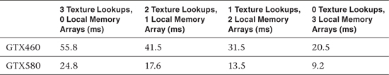
Table 19.1 shows the performance of the OpenCL optical flow algorithm. Using the radius and iterations shown previously, the GPU LK optical flow pipeline is able to process the test 640×480 “MiniCooper” image in 20.5ms on a GTX 460, which contains 7 multiprocessors. On a GTX 580 with 16 multiprocessors the same test took 9.2ms. The application of local memory made a significant difference, which could be seen by using either local memory or texture lookups for the image data.
Table 19.1 GPU Optical Flow Performance