
Chapter 18. Simulating the Ocean with Fast Fourier Transform
By Benedict R. Gaster,
Brian Sumner,
and Justin Hensley
Ocean is an OpenCL demonstration application developed at AMD that simulates the surface of the ocean in real time using an approach developed by Jerry Tessendorf1 that makes use of the fast Fourier transform (FFT). This same approach has been used in a number of feature films such as Waterworld, Titanic, and Fifth Element and has also appeared in modified form in real-time games. Briefly, the fast Fourier transform is applied to random noise, generated using the Phillips spectrum that evolves over time as a frequency-dependent phase shift. In this chapter we describe our implementation of Tessendorf’s approach and its application in AMD’s Ocean demo. An example frame generated by this application appears in grayscale2 in Figure 18.1 and in full color on the front cover of the book.
Figure 18.1 A single frame from the Ocean demonstration
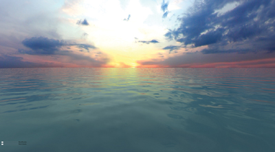
A key goal of this chapter is to describe an implementation of an optimized fast Fourier transform in OpenCL, but we have chosen to frame it within the Ocean application to show a “real” use case. We do not discuss the OpenGL rendering (it is mostly orthogonal to our main focus) except when it pertains to OpenCL/OpenGL interoperability.
An Overview of the Ocean Application
The application consists of two major components:
• The OpenCL generation of a height map, updated in each frame to account for the movement of waves
• The OpenGL rendering of this height map to produce the output, as seen in Figure 18.1
The program itself is a simple GLUT application (www.opengl.org/resources/libraries/glut/) that performs the following steps:
1. Initializes base OpenGL (which must be at least version 2.0 or above). No OpenGL objects are created at this time; this gives the application the flexibility to use interop between OpenGL and OpenCL or not. This choice is delayed until after OpenCL has initialized.
2. Initializes base OpenCL; creates a context, programs, and command-queues. At this time it also generates an initial spectrum that will be used in the simulation, with default wind direction and velocity. (The wind and velocity can be set by the user at any time during the simulation.)
3. Loads OpenGL textures, used for the sky box, logos, and so forth; loads and compiles OpenGL shaders; and creates a vertex buffer that will be used for interop with OpenCL if this feature is enabled.
4. Creates OpenCL buffers that will be used to store the resulting height map and are interop buffers with OpenGL, if that mode is enabled. Two buffers are produced by OpenCL that are used during rendering, the height map and a corresponding set of slopes used for calculating normals.
5. Finally the application enters the GLUT display loop, which is no different from most GLUT applications. The display callback itself is composed of the following elements:
a. Calls OpenCL to perform the next step in the simulation and produce vertex buffer data for the height map and corresponding slopes.
b. Renders the sky box.
c. Binds and renders the vertex buffers to produce the water, with respect to the sky box and other elements.
d. Finally, renders the controls for wind direction and velocity and the logo.
The OpenCL host code uses the C++ Wrapper API and is straightforward. We omit the initialization code here.
Each display iteration calls the following function:
cl_int runCLSimulation(
unsigned int width,
unsigned int height,
float animTime)
{
cl_int err;
std::vector<cl::Memory> v;
v.push_back(real);
v.push_back(slopes);
err = queue.enqueueAcquireGLObjects(&v);
checkErr(err, "Queue::enqueueAcquireGLObjects()");
err = generateSpectrumKernel.setArg(1, real);
err |= generateSpectrumKernel.setArg(3, width);
err |= generateSpectrumKernel.setArg(4, height);
err |= generateSpectrumKernel.setArg(5, animTime);
err |= generateSpectrumKernel.setArg(6, _patchSize);
checkErr(err, "Kernel::setArg(generateSpectrumKernel)");
err = queue.enqueueNDRangeKernel(
generateSpectrumKernel,
cl::NullRange,
cl::NDRange(width+64,height),
cl::NDRange(8,8));
checkErr(
err,
"CommandQueue::enqueueNDRangeKernel"
" (generateSpectrumKernel)");
err = kfftKernel.setArg(0, real);
err = queue.enqueueNDRangeKernel(
kfftKernel,
cl::NullRange,
cl::NDRange(FFT_SIZE*64),
cl::NDRange(64));
checkErr(
err,
"CommandQueue::enqueueNDRangeKernel(kfftKernel1)");
err = ktranKernel.setArg(0, real);
err = queue.enqueueNDRangeKernel(
ktranKernel,
cl::NullRange,
cl::NDRange(256*257/2 * 64),
cl::NDRange(64));
checkErr(
err,
"CommandQueue::enqueueNDRangeKernel(ktranKernel1)");
err = queue.enqueueNDRangeKernel(
kfftKernel,
cl::NullRange,
cl::NDRange(FFT_SIZE*64),
cl::NDRange(64));
checkErr(
err,
"CommandQueue::enqueueNDRangeKernel(kfftKernel2)");
err = calculateSlopeKernel.setArg(0, real);
err |= calculateSlopeKernel.setArg(1, slopes);
err |= calculateSlopeKernel.setArg(2, width);
err |= calculateSlopeKernel.setArg(3, height);
checkErr(err, "Kernel::setArg(calculatSlopeKernel)");
err = queue.enqueueNDRangeKernel(
calculateSlopeKernel,
cl::NullRange,
cl::NDRange(width,height),
cl::NDRange(8,8));
checkErr(err,
"CommandQueue::enqueueNDRangeKernel(calculateSlopeKernel)");
err = queue.enqueueReleaseGLObjects(&v);
checkErr(err, "Queue::enqueueReleaseGLObjects()");
queue.finish();
return CL_SUCCESS;
}
The runCLSimulation function is straightforward and is composed of the following steps:
1. Acquires shared OpenGL objects, enforcing the OpenCL and OpenGL parts of the application to be in sync.
2. Time-steps the FFT spectrum, representing the transformed height field of the ocean. This is outlined in the next section, “Phillips Spectrum Generation.”
3. Performs the inverse Fourier transform of the height field, outlined in detail later in the section “An OpenCL Discrete Fourier Transform.”
4. Calculates slopes from the height map (used for normal generation in the rendering).
5. Releases shared OpenGL objects, enforcing the OpenCL and OpenGL parts of the application to again be in sync.
Phillips Spectrum Generation
To generate an initial (noise) distribution and account for wind direction and velocity, that inverse discrete fast Fourier transform (DFFT) is then applied to simulate the motion over time. We use a kernel to apply the Phillips spectrum. A detailed description of why this is a good choice is beyond the scope of this book; the interested reader is directed to Tessendorf’s work.3 The Phillips spectrum is used to decide wave amplitudes at different (spatial or temporal) frequencies:
phillips(K) = A (exp (-1 / sqrt(kL)^2 / k^4) mag(norm(K) dot norm(w))^2
where
• k is the magnitude of K (the wave vector), which is 2 pi/lambda, where lambda is the length of the wave
• A is a constant globally affecting wave height
• L is v^2/g, which is the largest possible wave arising from a continuous wind with speed v, where gravitational constant g = 9.81
• norm(w) is the normalized wind vector (i.e., wind direction), and norm(K) is the normalized wave vector (i.e., wave direction)
The expression mag(norm(K) dot norm(w))^2 reduces a wave’s magnitude that is moving perpendicular to the wind, while allowing ones that move against it.
As this initial step of generating the Phillips spectrum is computed only once for wind direction and velocity, we choose to implement this step on the host, and then at each stage of the simulation we perform the final step into the FFT spectrum, with respect to time, in OpenCL. Taking this approach avoids having to provide an OpenCL C random number generator; we saw this step as orthogonal, and because there was little to no performance impact it seemed unnecessary. However, it is also worth pointing out that just because we could do something in OpenCL it does not mean that we should; in this case it seemed that the additional work when traded off against the performance gain really could not be justified. The host code to perform this is as follows:
float phillips(
float kx,
float ky,
float
windSpeed,
float windDirection)
{
float fWindDir = windDirection * OPENCL_PI_F / 180.0f;
static float A = 2.f*.00000005f;
float L = windSpeed * windSpeed / 9.81f;
float w = L / 75;
float ksqr = kx * kx + ky * ky;
float kdotwhat = kx * cosf(fWindDir) + ky * sinf(fWindDir);
kdotwhat = max(0.0f, kdotwhat);
float result =
(float) (A * (pow(2.7183f, -1.0f / (L * L * ksqr))
* (kdotwhat * kdotwhat)) / (ksqr * ksqr * ksqr));
float damp = (float) expf(-ksqr * w * w);
damp = expf(-1.0 / (ksqr * L * L));
result *= kdotwhat < 0.0f ? 0.25f : 1.0f;
return (result * damp);
}
This function is called for each kx and ky in the height field, whose dimensions are chosen to match the supported FFT dimensions. In this chapter we descibe a 1K×1K FFT implementation but the Ocean application itself supports the additional 2K×2K mode.
The following applies the phillips function to each position in the input space to produce an initial height field, with respect to the given wind speed and direction:
void generateHeightField(
cl_float2 * h0,
unsigned int fftInputH,
unsigned int fftInputW)
{
float fMultiplier, fAmplitude, fTheta;
for (unsigned int y = 0; y<fftInputH; y++) {
for (unsigned int x = 0; x<fftInputW; x++) {
float kx = OPENCL_PI_F * x / (float) _patchSize;
float ky = 2.0f * OPENCL_PI_F * y / (float) _patchSize;
float Er = 2.0f * rand() / (float) RAND_MAX - 1.0f;
float Ei = 2.0f * rand() / (float) RAND_MAX - 1.0f;
if (!((kx == 0.f) && (ky == 0.f))) {
fMultiplier = sqrt(phillips(kx,ky,windSpeed, windDir));
}
else {
fMultiplier = 0.f;
}
fAmplitude = RandNormal(0.0f, 1.0f);
fTheta = rand() / (float) RAND_MAX * 2 * OPENCL_PI_F;
float h0_re = fMultiplier * fAmplitude * Er;
float h0_im = fMultiplier * fAmplitude * Ei;
int i = y*fftInputW+x;
cl_float2 tmp = {h0_re, h0_im};
h0[i] = tmp;
}
}
}
Finally, the following OpenCL kernel, along with two support functions, updates the spectrum on each iteration of the simulation, with respect to time, thus providing movement:
// complex math functions
float2 __attribute__((always_inline)) conjugate(float2 arg)
{
return (float2)(arg.x, -arg.y);
}
float2 __attribute__((always_inline)) complex_exp(float arg)
{
float s;
float c;
s = sincos(arg, &c);
return (float2)(c,s);
}
__kernel void generateSpectrumKernel(
__global float2* h0,
__global float * ht_real,
__global float * ht_imag,
unsigned int width,
unsigned int height,
float t,
float patchSize)
{
size_t x = get_global_id(0);
size_t y = get_global_id(1);
unsigned int i = y*width+x;
// calculate coordinates
float2 k;
k.x = M_PI * x / (float) patchSize;
k.y = 2.0f * M_PI * y / (float) patchSize;
// calculate dispersion w(k)
float k_len = length (k);
float w = sqrt(9.81f * k_len);
float2 h0_k = h0[i];
float2 h0_mk = h0[(((height-1)-y)*width)+x];
float2 h_tilda = complex_mult(
h0_k,
complex_exp(w * t)) +
complex_mult(conjugate(h0_mk), complex_exp(-w * t));
// output frequency-space complex values
if ((x < width) && (y < height)) {
ht_real[i] = h_tilda.x;
ht_imag[i] = h_tilda.y;
}
}
An OpenCL Discrete Fourier Transform
The discrete Fourier transform (DFT) is an extremely important operation in many fields because of its many special properties such as replacing convolution with pointwise multiplication4 and very fast implementations.5 Additionally, there are a number of very high-quality and high-performance implementations for the CPU, such as FFTW (http://fftw.org).
There are fewer implementations and less information available on producing efficient FFTs for OpenCL GPU devices. In the following sections we will walk through the detailed thinking behind the Ocean application and the resulting code used in it. While these sections are mostly focused on transforms of size 1024, we expect this kind of analysis to be quite useful for other sizes as well.
Determining 2D Decomposition
While it is possible to decompose a 2D FFT into smaller 2D FFTs followed by a “recombination” step, we will instead use the following usual approach to achieve the 2D transform:
1. Transform all rows using 1D FFT.
2. Transform all columns using 1D FFT.
However, for many memory systems, the accesses made in step 2 can suffer performance problems. We can investigate this on the GPU by timing two OpenCL kernels that add a constant to each element of a 1K×1K float array. The first kernel assigns a work-group to each row of the array, and the second assigns a work-group to each column. The elapsed times (in milliseconds) observed for each kernel for a few different work-group sizes are shown in Table 18.1.
Table 18.1 Kernel Elapsed Times for Varying Work-Group Sizes
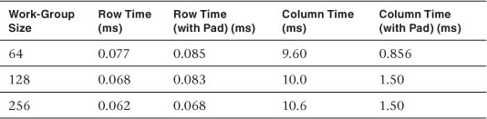
The smallest row time of 0.062ms indicates that we were achieving a round-trip bandwidth of 133GB per second. The second (pad) time listed for each kernel shows the effect of adding a number of “pad” columns (64 on the device we used to obtain the timings) to improve the performance of the memory system. On the CPU, such padding is often done to reduce the effects of cache thrashing; on the GPU, padding can help spread the accesses over more memory controllers.
The large difference between the row time and column time suggests an alternative approach:
1. Transform all rows using 1D FFT.
2. Transpose 1K×1K array.
3. Transform all rows using 1D FFT.
4. Transpose 1K×1K array.
This can be faster than the first approach if the transpose can be performed quickly enough. Note that in the Ocean code, one of the transposes can be eliminated by simply constructing the data in transposed order. Similarly, leaving the result of a 2D FFT in transposed order is a typical option in FFT packages to improve performance.
Using Local Memory
A 1D FFT is usually carried out as a series of “passes” over the data. For instance, we can recursively expand the decimation-in-time binary decomposition until the transform length is 2 (where W is a diagonal array of roots of unity usually called “twiddle factors”):
Outlo = FFT(Ineven) + W FFT(Inodd)
Outhi = FFT(Ineven) − W FFT(Inodd)
Thus we arrive at a procedure that requires ten passes over the data (1024 = 210):
Out0 = Pass0(In)
Out1 = Pass1(Out0)
Out = Pass9(Out8)
Without local memory each pass requires a round trip of data from global memory. Also, element access during the pass may not hit the memory system efficiently.
Of course, the number of passes can be reduced by stopping the recursion earlier. Two passes of length 32 FFT would also work, as would five passes of length 4 FFT, as well as two passes of length 16 FFT followed by one pass of length 4. There are trade-offs with each of these choices, as we will see.
When local memory is used, some fraction of the data to be transformed is kept in local memory, and transfers to and from global memory may be reduced to just a few passes, such as the first and last passes. Other passes will read and write local memory, which, being on chip, is much faster than global memory. However, local memory is also a limited hardware resource and constrains the number of work-groups that can use it concurrently. This constraint directly affects the number of work-items in flight and hence the latency-hiding ability of the GPU.
For the Ocean 1K FFT we chose to make use of local memory to reduce the global memory traffic to just the first and last passes.
Determining the Sub-Transform Size
As mentioned previously, the amount of local memory used by a kernel constrains the number of work-items in flight. Another constraint is imposed by the number of physical registers used. Roughly speaking, the larger the number used, the fewer the work-items in flight. OpenCL C does not provide direct control over register use, but it can be controlled indirectly by the choice of algorithm and implementation of that algorithm.
A sub-transform of length R requires around 2R registers. However, near-optimal operation count short DFTs may require several more than 2R registers depending on the compiler. With register utilization figuring so prominently in latency hiding, it makes sense to look for minimal register implementations for a given R.
Using larger Rs means fewer passes but also potentially fewer work-items in flight. An FFT library should seek the best trade-off of these effects to achieve the best performance.
In the Ocean code, we chose to decompose the 1K FFT into five passes of length 4 sub-transforms (1024 = 45). A 4-point DFT can be computed in place with no additional registers:
ar0 = zr0 + zr2;
br1 = zr0 - zr2;
ar2 = zr1 + zr3;
br3 = zr1 - zr3;
zr0 = ar0 + ar2;
zr2 = ar0 - ar2;
ai0 = zi0 + zi2;
bi1 = zi0 - zi2;
ai2 = zi1 + zi3;
bi3 = zi1 - zi3;
zi0 = ai0 + ai2;
zi2 = ai0 - ai2;
zr1 = br1 + bi3;
zi1 = bi1 - br3;
zr3 = br1 - bi3;
zi3 = br3 + bi1;
The inputs and outputs here are zr0...zr3 (real components) and zi0...zi3 (imaginary components). Unfortunately, post-multiplication by the twiddle factors requires a few more registers to hold the twiddle factor(s) and intermediate results of the complex multiplication.
Determining the Work-Group Size
An OpenCL FFT kernel can adapt itself to the work-group size it is presented with at the cost of significant logic and indexing complexity. Alternatively, control flow can be completely eliminated and indexing computation greatly reduced by using a kernel targeted for a specific transform length and work-group size. The most efficient work-group sizes are usually multiples of the hardware wavefront/warp size.
In the Ocean code, for our 1K length we use a work-group to process a single transform and considered work-group sizes of 64, 128, and 256. For work-group size 64, each work-item must process 16 points per pass, that is, four 4-point DFTs (which can be conveniently expressed using OpenCL C’s float4 type). For work-group size 128, each work-item must process 8 points per pass, and for work-group size 256, each work-item must process 4 points per pass. Of course, “points” is proportional to “registers,” so the work-group size gives us a knob to adjust work-item register use. However, the number of registers used by the entire work-group does not change.
For the Ocean code, we chose the smaller work-group size of 64.
Obtaining the Twiddle Factors
The twiddle factors used in the FFT are a key ingredient in combining smaller transforms into larger ones. They are primitive nth roots of unity (or simple functions thereof) and are of the form cos(A) + i sin(A) (where i is the imaginary value sqrt(-1) and A is 2 pi K/N, where N is the transform length and 0 <= K < N). There are a variety of options for obtaining the twiddle factors affecting both performance and accuracy. They can be computed by the accurate OpenCL built-in sin and cos functions. They can instead be computed using either the built-in half_sin and half_cos functions or the built-in native_sin and native_cos functions. GPUs typically have limited-accuracy machine instructions for sine and cosine that are exposed by the native_sin and native_cos built-in functions. They can offer the highest performance, but the cost is reduced accuracy of the result.
Other options are to read precomputed twiddle factors from a constant buffer, image (texture), or global buffer. The first two are likely to be faster than the third because of caching, and the first can be used especially easily by simply defining a simple OpenCL __constant array in the kernel program itself.
It is also worth noting that a combination of approaches of varying accuracy may also be used based on various instances of the “double angle” formulas of trigonometry.
For the Ocean code, we decided that the accuracy of the native functions was sufficient.
Determining How Much Local Memory Is Needed
In each pass, a given work-item may require data produced by a different work-item on the previous pass. Local or global memory is needed to pass data between work-items, and we’ve determined that we’ll use local memory. We can trade off between local memory size and complexity and number of barriers.
For instance, in the simplest (maximum use) case, a pass would look like this:
1. Load entire vector from local memory into registers.
2. Local barrier.
3. Compute sub-transform(s).
4. Save entire vector to local memory.
5. Local barrier.
If the entire vector is able to be held in registers, we can halve the amount of local memory needed by partially mixing passes into this:
1. Compute sub-transforms.
2. Save real part of vector to local memory.
3. Local barrier.
4. Read next pass real part of vector from local memory.
5. Local barrier.
6. Save imaginary part of vector to local memory.
7. Local barrier.
8. Read next pass imaginary part of vector from local memory.
It may be possible to reduce the amount of local memory even further by writing and reading subsets of the vector, along with more barriers.
In the Ocean code, we use the second approach and note that all the local barriers are essentially free because the work-group size we chose is the same as the wavefront size on the GPU hardware we are using.
Avoiding Local Memory Bank Conflicts
Local memories are often banked structures, and performance may be reduced when the work-group/wavefront/warp accesses only a small number of memory banks on a given access. There are a number of techniques to reduce conflicts, including more complicated addressing and/or padding.
Of course, padding can increase the amount of memory used by the kernel and end up degrading the ability of the GPU to hide latency, so ideally both cases should be compared.
For the Ocean code, we found that a transpose implementation with local memory bank conflicts performs at about the same speed as a conflict-free version. However, for the FFT, we found that a conflict-free implementation is about 61 percent faster than a version with conflicts.
Using Images
Up to this point, we have been assuming that the inputs and outputs of the FFT and transpose kernels have been OpenCL buffers. However, the inputs could instead be OpenCL read-only images (usually cached) and write-only images that are accessed using OpenCL samplers. If we consider the multipass structure of the FFT, though, the only significant differences in the implementation would be the initial read of data from the input image and the final store to the output image. The situation would be different if OpenCL were to ever allow read-write images.
A Closer Look at the FFT Kernel
The FFT kernel starts with this:
__kernel __attribute__((reqd_work_group_size (64,1,1))) void
kfft(__global float *greal, __global float *gimag)
{
// This is 4352 bytes
__local float lds[1088];
This tells us a few things already:
• The kernel is designed specifically for a 1D iteration space with a work-group size of 64.
• The real and imaginary parts of the complex data are in separate arrays rather than interleaved within a single array. (This turns out to be most convenient for the rest of the Ocean code.)
• Because there are no other arguments, this kernel was designed for only one FFT size (1K).
• Some padding must be in use because 1088 is not the 1024 or 2048 that we might expect.
This kernel gets to pulling in the data pretty quickly:
uint gid = get_global_id(0);
uint me = gid & 0x3fU;
uint dg = (me << 2) + (gid >> 6) * VSTRIDE;
__global float4 *gr = (__global float4 *)(greal + dg);
__global float4 *gi = (__global float4 *)(gimag + dg);
float4 zr0 = gr[0*64];
float4 zr1 = gr[1*64];
float4 zr2 = gr[2*64];
float4 zr3 = gr[3*64];
float4 zi0 = gi[0*64];
float4 zi1 = gi[1*64];
float4 zi2 = gi[2*64];
float4 zi3 = gi[3*64];
Here, VSTRIDE is the number of elements between the first element of two successive rows. Each access to gr and gi pulls 1024 consecutive bytes from the vector being worked on, and each work-item gets four consecutive elements of the vector, each set of four separated by 256 elements, which is exactly what is required for the first pass of a length 4 sub-transform pass.
The first transform and multiplication by twiddle factor appear as
FFT4();
int4 tbase4 = (int)(me << 2) + (int4)(0, 1, 2, 3);
TW4IDDLE4();
The 4-point FFT was given previously when we determined the sub-transform size. Because the type of the variables is float4, the kernel must use at least 32 registers. We recall from when we obtained our twiddle factors that the twiddle factor “angle” is a multiple of 2 pi/1024. The specific multiple required by the first pass is given by the tbase4 computation. The actual computation of the twiddle factors is carried out by the following function, where ANGLE is 2 pi/1024:
__attribute__((always_inline)) float4
k_sincos4(int4 i, float4 *cretp)
{
i -= (i > 512) & 1024;
float4 x = convert_float4(i) * -ANGLE;
*cretp = native_cos(x);
return native_sin(x);
}
The first statement in the function quickly and accurately reduces the range of the angle to the interval [-pi, pi].
Following the actual computation, each work-item needs to save the values it has produced and read the new ones it needs for the next pass. Let’s look at a single store and load at the end of the first pass:
__local float *lp = lds + ((me << 2) + (me >> 3));
lp[0] = zr0.x;
...
barrier(CLK_LOCAL_MEM_FENCE);
lp = lds + (me + (me >> 5));
zr0.x = lp[0*66];
Each store to or load from lp is of course a SIMD parallel operation. The local memory on the GPU we used has 32 banks of 32-bit values. Using the previous addressing expressions, we can compute the first several load and store banks, as shown in Table 18.2.
Table 18.2 Load and Store Bank Calculations
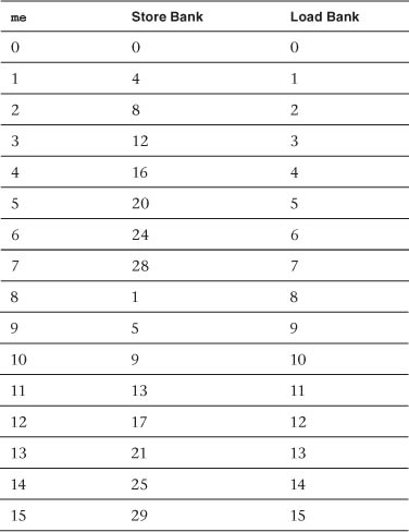
It turns out that all 64 work-items in the work-group access each bank exactly twice on each load and store, which is optimal.
The following four passes look very much like the first with the exception that the twiddle factors vary more slowly and the addressing into local memory changes because of the different elements needed for each pass. In each case the addressing has been chosen to minimize bank conflicts.
In the last pass, the twiddle factors are all 1.0, so the final sub-transform and store back to global memory looks like the following, where again each store transfers 1024 consecutive bytes back to global memory:
FFT4();
gr[0*64] = zr0;
gr[1*64] = zr1;
gr[2*64] = zr2;
gr[3*64] = zr3;
gi[0*64] = zi0;
gi[1*64] = zi1;
gi[2*64] = zi2;
gi[3*64] = zi3;
On the GPU we tested, transforming 1024 vectors using this kernel takes about 0.13ms. Using the standard 5 N log2(N) approximation for the flop count for an FFT of length N, this time corresponds to a rate of about 400 GFLOPS per second. It also corresponds to a round-trip bandwidth from global memory of about 130GB per second.
A Closer Look at the Transpose Kernel
The transpose kernel is responsible for transposing the two 1024×1024 arrays that make up the complex data. Because these arrays are square, the operation can be performed in place quite easily. As one might expect, we break the arrays into smaller blocks. Each work-group is then assigned a pair of blocks, (i, j) and (j, i), which are then read into local memory and transposed. Block (i, j) is then stored to location (j, i), and block (j, i) is stored to location (i, j). We evaluated a few different block sizes and settled on a 32×32 block for the Ocean code.
One small question arises: how to assign a block to a work-group, because operating on all blocks as previously described would only end up transposing the diagonal blocks. We make use of a convenient quadratic polynomial:
pB(t) = - ½ t2 + (B + ½) t
At the non-negative integers, this polynomial takes on the values 0, B, B + (B - 1), B + (B - 1) + (B - 2), and so on. Given our 32×32 block size, if we choose B = 1024/32 = 32, we can compute (i, j) using this code found in the transpose kernel:
uint gid = get_global_id(0);
uint me = gid & 0x3fU;
uint k = gid >> 6;
int l = 32.5f - native_sqrt(1056.25f - 2.0f * (float)as_int(k));
int kl = ((65 - l) * l) >> 1;
uint j = k - kl;
uint i = l + j;
The blocks accessed run down the diagonal and then the subdiagonals.
Given our work-group size of 64, each work-item must handle 16 points of the block. The block is read using
uint go = ((me & 0x7U) << 2) + (me >> 3)*VSTRIDE;
uint goa = go + (i << 5) + j * (VSTRIDE*32);
uint gob = go + (j << 5) + i * (VSTRIDE*32);
__global float4 *gp = (__global float4 *)(greal + goa);
float4 z0 = gp[0*VSTRIDE/4*8];
float4 z1 = gp[1*VSTRIDE/4*8];
float4 z2 = gp[2*VSTRIDE/4*8];
float4 z3 = gp[3*VSTRIDE/4*8];
We’ve assigned the threads so that each access fetches eight 256-byte chunks of global memory.
The transpose in the Ocean code uses the conflict-free approach. So just as for the FFT, the addressing of loads and stores to local memory is slightly complicated. The first store and load looks like this:
uint lo = (me >> 5) + (me & 0x7U)*9 + ((me >> 3) & 0x3U)*(9*8);
__local float *lp = ldsa + lo;
lp[0*2] = z0.x;
...
barrier(CLK_LOCAL_MEM_FENCE);
uint lot = (me & 0x7U) + ((me >> 3) & 0x3U)*
(9*8*4 + 8) + (me >> 5)*9;
lp = ldsa + lot;
z0.x = lp[0*2*9];
Once again, these accesses are optimal. Data is written back to global memory in the same eight 256-byte chunks per access.
On the machine we tested, using a VSTRIDE of 1088, the Ocean transpose kernel runs in about 0.14ms, which corresponds to a round-trip bandwidth to global memory of about 120GB per second.
Thus, the time for the entire 2D FFT used in Ocean is roughly 0.13 + 0.14 + 0.13 = 0.40 ms.