Chapter 1. An Introduction to OpenCL

When learning a new programming model, it is easy to become lost in a sea of details. APIs and strange new terminology seemingly appear from nowhere, creating needless complexity and sowing confusion. The key is to begin with a clear high-level understanding, to provide a map to fall back on when the going gets tough.

The purpose of this chapter is to help you construct that map. We begin with a brief overview of the OpenCL 1.1 specification and the heterogeneous computing trends that make it such an important programming standard. We then describe the conceptual models behind OpenCL and use them to explain how OpenCL works. At this point, the theoretical foundation of OpenCL is established, and we move on to consider the components of OpenCL. A key part of this is how OpenCL works with graphics standards. We complete our map of the OpenCL landscape by briefly looking at how the OpenCL standard works with embedded processors.

What Is OpenCL, or . . . Why You Need This Book

OpenCL is an industry standard framework for programming computers composed of a combination of CPUs, GPUs, and other processors. These so-called heterogeneous systems have become an important class of platforms, and OpenCL is the first industry standard that directly addresses their needs. First released in December of 2008 with early products available in the fall of 2009, OpenCL is a relatively new technology.

With OpenCL, you can write a single program that can run on a wide range of systems, from cell phones, to laptops, to nodes in massive supercomputers. No other parallel programming standard has such a wide reach. This is one of the reasons why OpenCL is so important and has the potential to transform the software industry. It’s also the source of much of the criticism launched at OpenCL.

OpenCL delivers high levels of portability by exposing the hardware, not by hiding it behind elegant abstractions. This means that the OpenCL programmer must explicitly define the platform, its context, and how work is scheduled onto different devices. Not all programmers need or even want the detailed control OpenCL provides. And that’s OK; when available, a high-level programming model is often a better approach. Even high-level programming models, however, need a solid (and portable) foundation to build on, and OpenCL can be that foundation.

This book is a detailed introduction to OpenCL. While anyone can download the specification (www.khronos.org/opencl) and learn the spelling of all the constructs within OpenCL, the specification doesn’t describe how to use OpenCL to solve problems. That is the point of this book: solving problems with the OpenCL framework.

Our Many-Core Future: Heterogeneous Platforms

Computers over the past decade have fundamentally changed. Raw performance used to drive innovation. Starting several years ago, however, the focus shifted to performance delivered per watt expended. Semiconductor companies will continue to squeeze more and more transistors onto a single die, but these vendors will compete on power efficiency instead of raw performance.

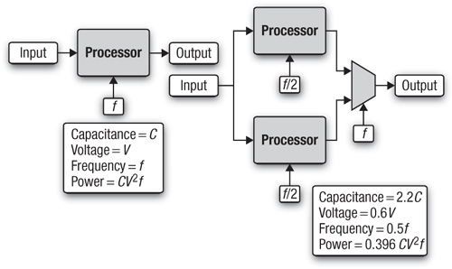
This shift has radically changed the computers the industry builds. First, the microprocessors inside our computers are built from multiple low-power cores. The multicore imperative was first laid out by A. P. Chandrakasan et al. in the article “Optimizing Power Using Transformations.”¹ The gist of their argument can be found in Figure 1.1. The energy expended in switching the gates in a CPU is the capacitance (C) times the voltage (V) squared. These gates switch over the course of a second a number of times equal to the frequency. Hence the power of a microprocessor scales as P = CV²f. If we compare a single-core processor running at a frequency of f and a voltage of V to a similar processor with two cores each running at f/2, we have increased the number of circuits in the chip. Following the models described in “Optimizing Power Using Transformations,” this nominally increases the capacitance by a factor of 2.2. But the voltage drops substantially to 0.6V. So the number of instructions retired per second is the same in both cases, but the power in the dual-core case is 0.396 of the power for the single-core. This fundamental relationship is what is driving the transition to many-core chips. Many cores running at lower frequencies are fundamentally more power-efficient.

Figure 1.1 The rate at which instructions are retired is the same in these two cases, but the power is much less with two cores running at half the frequency of a single core.

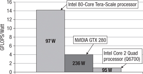
The next question is “Will these cores be the same (homogeneous) or will they be different?” To understand this trend, consider the power efficiency of specialized versus general-purpose logic. A general-purpose processor by its nature must include a wide range of functional units to respond to any computational demand. This is precisely what makes the chip a general-purpose processor. Processors specialized to a specific function, however, have fewer wasted transistors because they include only those functional units required by their special function. The result can be seen in Figure 1.2, where we compare a general-purpose CPU (Intel Core 2 Quad processor model Q6700),² a GPU (NVIDIA GTX 280),³ and a highly specialized research processor (Intel 80-core Tera-scale research processor, the cores of which are just a simple pair of floating-point multiply-accumulate arithmetic units).⁴ To make the comparisons as fair as possible, each of the chips was manufactured with a 65nm process technology, and we used the vendor-published peak performance versus thermal design point power. As plainly shown in the figure, as long as the tasks are well matched to the processor, the more specialized the silicon the better the power efficiency.

Figure 1.2 A plot of peak performance versus power at the thermal design point for three processors produced on a 65nm process technology. Note: This is not to say that one processor is better or worse than the others. The point is that the more specialized the core, the more power-efficient it is.

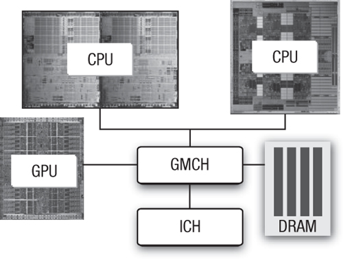
Hence, there is good reason to believe that in a world where maximizing performance per watt is essential, we can expect systems to increasingly depend on many cores with specialized silicon wherever practical. This is especially important for mobile devices in which conservation of battery power is critical. This heterogeneous future, however, is already upon us. Consider the schematic representation of a modern PC in Figure 1.3. There are two sockets, each potentially holding a different multicore CPU; a graphics/memory controller (GMCH) that connects to system memory (DRAM); and a graphics processing unit (GPU). This is a heterogeneous platform with multiple instruction sets and multiple levels of parallelism that must be exploited in order to utilize the full potential of the system.

Figure 1.3 Block diagram of a modern desktop PC with multiple CPUs (potentially different) and a GPU, demonstrating that systems today are frequently heterogeneous

The basic platform, both today and in the future, at a high level is clear. A host of details and innovations will assuredly surprise us, but the hardware trends are clear. The future belongs to heterogeneous many-core platforms. The question facing us is how our software should adapt to these platforms.

Software in a Many-Core World

Parallel hardware delivers performance by running multiple operations at the same time. To be useful, parallel hardware needs software that executes as multiple streams of operations running at the same time; in other words, you need parallel software.

To understand parallel software, we must begin with the more general concept of concurrency. Concurrency is an old and familiar concept in computer science. A software system is concurrent when it consists of more than one stream of operations that are active and can make progress at one time. Concurrency is fundamental in any modern operating system. It maximizes resource utilization by letting other streams of operations (threads) make progress while others are stalled waiting on some resource. It gives a user interacting with the system the illusion of continuous and near-instantaneous interaction with the system.

When concurrent software runs on a computer with multiple processing elements so that threads actually run simultaneously, we have parallel computation. Concurrency enabled by hardware is parallelism.

The challenge for programmers is to find the concurrency in their problem, express that concurrency in their software, and then run the resulting program so that the concurrency delivers the desired performance. Finding the concurrency in a problem can be as simple as executing an independent stream of operations for each pixel in an image. Or it can be incredibly complicated with multiple streams of operations that share information and must tightly orchestrate their execution.

Once the concurrency is found in a problem, programmers must express this concurrency in their source code. In particular, the streams of operations that will execute concurrently must be defined, the data they operate on associated with them, and the dependencies between them managed so that the correct answer is produced when they run concurrently. This is the crux of the parallel programming problem.

Manipulating the low-level details of a parallel computer is beyond the ability of most people. Even expert parallel programmers would be overwhelmed by the burden of managing every memory conflict or scheduling individual threads. Hence, the key to parallel programming is a high-level abstraction or model to make the parallel programming problem more manageable.

There are way too many programming models divided into overlapping categories with confusing and often ambiguous names. For our purposes, we will worry about two parallel programming models: task parallelism and data parallelism. At a high level, the ideas behind these two models are straightforward.

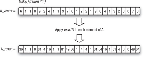
In a data-parallel programming model, programmers think of their problems in terms of collections of data elements that can be updated concurrently. The parallelism is expressed by concurrently applying the same stream of instructions (a task) to each data element. The parallelism is in the data. We provide a simple example of data parallelism in Figure 1.4. Consider a simple task that just returns the square of an input value and a vector of numbers (A_vector). Using the data-parallel programming model, we update the vector in parallel by stipulating that the task be applied to each element to produce a new result vector. Of course, this example is extremely simple. In practice the number of operations in the task must be large in order to amortize the overheads of data movement and manage the parallel computation. But the simple example in the figure captures the key idea behind this programming mode.

Figure 1.4 A simple example of data parallelism where a single task is applied concurrently to each element of a vector to produce a new vector

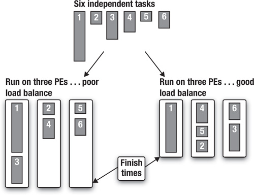
In a task-parallel programming model, programmers directly define and manipulate concurrent tasks. Problems are decomposed into tasks that can run concurrently, which are then mapped onto processing elements (PEs) of a parallel computer for execution. This is easiest when the tasks are completely independent, but this programming model is also used with tasks that share data. The computation with a set of tasks is completed when the last task is done. Because tasks vary widely in their computational demands, distributing them so that they all finish at about the same time can be difficult. This is the problem of load balancing. Consider the example in Figure 1.5, where we have six independent tasks to execute concurrently on three PEs. In one case the first PE has extra work to do and runs significantly longer than the other PEs. The second case with a different distribution of tasks shows a more ideal case where each PE finishes at about the same time. This is an example of a key ideal in parallel computing called load balancing.

Figure 1.5 Task parallelism showing two ways of mapping six independent tasks onto three PEs. A computation is not done until every task is complete, so the goal should be a well-balanced load, that is, to have the time spent computing by each PE be the same.

The choice between data parallelism and task parallelism is driven by the needs of the problem being solved. Problems organized around updates over points on a grid, for example, map immediately onto data-parallel models. Problems expressed as traversals over graphs, on the other hand, are naturally expressed in terms of task parallelism. Hence, a well-rounded parallel programmer needs to be comfortable with both programming models. And a general programming framework (such as OpenCL) must support both.

Regardless of the programming model, the next step in the parallel programming process is to map the program onto real hardware. This is where heterogeneous computers present unique problems. The computational elements in the system may have different instruction sets and different memory architectures and may run at different speeds. An effective program must understand these differences and appropriately map the parallel software onto the most suitable OpenCL devices.

Traditionally, programmers have dealt with this problem by thinking of their software as a set of modules implementing distinct portions of their problem. The modules are explicitly tied to the components in the heterogeneous platform. For example, graphics software runs on the GPU. Other software runs on the CPU.

General-purpose GPU (GPGPU) programming broke this model. Algorithms outside of graphics were modified to fit onto the GPU. The CPU sets up the computation and manages I/O, but all the “interesting” computation is offloaded to the GPU. In essence, the heterogeneous platform is ignored and the focus is placed on one component in the system: the GPU.

OpenCL discourages this approach. In essence, a user “pays for all the OpenCL devices” in a system, so an effective program should use them all. This is exactly what OpenCL encourages a programmer to do and what you would expect from a programming environment designed for heterogeneous platforms.

Hardware heterogeneity is complicated. Programmers have come to depend on high-level abstractions that hide the complexity of the hardware. A heterogeneous programming language exposes heterogeneity and is counter to the trend toward increasing abstraction.

And this is OK. One language doesn’t have to address the needs of every community of programmers. High-level frameworks that simplify the programming problem map onto high-level languages, which in turn map to a low-level hardware abstraction layer for portability. OpenCL is that hardware abstraction layer.

Conceptual Foundations of OpenCL

As we will see later in this book, OpenCL supports a wide range of applications. Making sweeping generalizations about these applications is difficult. In every case, however, an application for a heterogeneous platform must carry out the following steps:

1. Discover the components that make up the heterogeneous system.

2. Probe the characteristics of these components so that the software can adapt to the specific features of different hardware elements.

3. Create the blocks of instructions (kernels) that will run on the platform.

4. Set up and manipulate memory objects involved in the computation.

5. Execute the kernels in the right order and on the right components of the system.

6. Collect the final results.

These steps are accomplished through a series of APIs inside OpenCL plus a programming environment for the kernels. We will explain how all this works with a “divide and conquer” strategy. We will break the problem down into the following models:

• Platform model: a high-level description of the heterogeneous system

• Execution model: an abstract representation of how streams of instructions execute on the heterogeneous platform

• Memory model: the collection of memory regions within OpenCL and how they interact during an OpenCL computation

• Programming models: the high-level abstractions a programmer uses when designing algorithms to implement an application

Platform Model

The OpenCL platform model defines a high-level representation of any heterogeneous platform used with OpenCL. This model is shown in Figure 1.6. An OpenCL platform always includes a single host. The host interacts with the environment external to the OpenCL program, including I/O or interaction with a program’s user.

Figure 1.6 The OpenCL platform model with one host and one or more OpenCL devices. Each OpenCL device has one or more compute units, each of which has one or more processing elements.

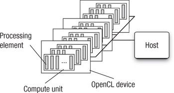
The host is connected to one or more OpenCL devices. The device is where the streams of instructions (or kernels) execute; thus an OpenCL device is often referred to as a compute device. A device can be a CPU, a GPU, a DSP, or any other processor provided by the hardware and supported by the OpenCL vendor.

The OpenCL devices are further divided into compute units which are further divided into one or more processing elements (PEs). Computations on a device occur within the PEs. Later, when we talk about work-groups and the OpenCL memory model, the reason for dividing an OpenCL device into processing elements and compute units will be clear.

Execution Model

An OpenCL application consists of two distinct parts: the host program and a collection of one or more kernels. The host program runs on the host. OpenCL does not define the details of how the host program works, only how it interacts with objects defined within OpenCL.

The kernels execute on the OpenCL devices. They do the real work of an OpenCL application. Kernels are typically simple functions that transform input memory objects into output memory objects. OpenCL defines two types of kernels:

• OpenCL kernels: functions written with the OpenCL C programming language and compiled with the OpenCL compiler. All OpenCL implementations must support OpenCL kernels.

• Native kernels: functions created outside of OpenCL and accessed within OpenCL through a function pointer. These functions could be, for example, functions defined in the host source code or exported from a specialized library. Note that the ability to execute native kernels is an optional functionality within OpenCL and the semantics of native kernels are implementation-defined.

The OpenCL execution model defines how the kernels execute. To explain this in detail, we break the discussion down into several parts. First we explain how an individual kernel runs on an OpenCL device. Because the whole point of writing an OpenCL application is to execute kernels, this concept is the cornerstone of understanding OpenCL. Then we describe how the host defines the context for kernel execution and how the kernels are enqueued for execution.

How a Kernel Executes on an OpenCL Device

A kernel is defined on the host. The host program issues a command that submits the kernel for execution on an OpenCL device. When this command is issued by the host, the OpenCL runtime system creates an integer index space. An instance of the kernel executes for each point in this index space. We call each instance of an executing kernel a work-item, which is identified by its coordinates in the index space. These coordinates are the global ID for the work-item.

The command that submits a kernel for execution, therefore, creates a collection of work-items, each of which uses the same sequence of instructions defined by a single kernel. While the sequence of instructions is the same, the behavior of each work-item can vary because of branch statements within the code or data selected through the global ID.

Work-items are organized into work-groups. The work-groups provide a more coarse-grained decomposition of the index space and exactly span the global index space. In other words, work-groups are the same size in corresponding dimensions, and this size evenly divides the global size in each dimension. Work-groups are assigned a unique ID with the same dimensionality as the index space used for the work-items. Work-items are assigned a unique local ID within a work-group so that a single work-item can be uniquely identified by its global ID or by a combination of its local ID and work-group ID.

The work-items in a given work-group execute concurrently on the processing elements of a single compute unit. This is a critical point in understanding the concurrency in OpenCL. An implementation may serialize the execution of kernels. It may even serialize the execution of work-groups in a single kernel invocation. OpenCL only assures that the work-items within a work-group execute concurrently (and share processor resources on the device). Hence, you can never assume that work-groups or kernel invocations execute concurrently. They indeed often do execute concurrently, but the algorithm designer cannot depend on this.

The index space spans an N-dimensioned range of values and thus is called an NDRange. Currently, N in this N-dimensional index space can be 1, 2, or 3. Inside an OpenCL program, an NDRange is defined by an integer array of length N specifying the size of the index space in each dimension. Each work-item’s global and local ID is an N-dimensional tuple. In the simplest case, the global ID components are values in the range from zero to the number of elements in that dimension minus one.

Work-groups are assigned IDs using a similar approach to that used for work-items. An array of length N defines the number of work-groups in each dimension. Work-items are assigned to a work-group and given a local ID with components in the range from zero to the size of the work-group in that dimension minus one. Hence, the combination of a work-group ID and the local ID within a work-group uniquely defines a work-item.

Let’s carefully work through the different indices implied by this model and explore how they are all related. Consider a 2D NDRange. We use the lowercase letter g for the global ID of a work-item in each dimension given by a subscript x or y. An uppercase letter G indicates the size of the index space in each dimension. Hence, each work-item has a coordinate (g_x, g_y) in a global NDRange index space of size (G_x, G_y) and takes on the values [0 .. (G_x - 1), 0 .. (G_y - 1)].

We divide the NDRange index space into work-groups. Following the conventions just described, we’ll use a lowercase w for the work-group ID and an uppercase W for the number of work-groups in each dimension. The dimensions are once again labeled by subscripts x and y.

OpenCL requires that the number of work-groups in each dimension evenly divide the size of the NDRange index space in each dimension. This way all work-groups are full and the same size. This size in each direction (x and y in our 2D example) is used to define a local index space for each work-item. We will refer to this index space inside a work-group as the local index space. Following our conventions on the use of uppercase and lowercase letters, the size of our local index space in each dimension (x and y) is indicated with an uppercase L and the local ID inside a work-group uses a lowercase l.

Hence, our NDRange index space of size G_x by G_y is divided into work-groups indexed over a W_x-by-W_y space with indices (w_x, w_y). Each work-group is of size L_x by L_y where we get the following:

L_x = G_x/W_x

L_y = G_y/W_y

We can define a work-item by its global ID (g_x, g_y) or by the combination of its local ID (l_x, l_y) and work-group ID (w_x, w_y):

g_x = w_x * L_x + l_x

g_y = w_y * L_y + l_y

Alternatively we can work backward from g_x and g_y to recover the local ID and work-group ID as follows:

w_x = g_x/L_x

w_y = g_y/L_y

l_x = g_x % L_x

l_y = g_y % L_y

In these equations we used integer division (division with truncation) and the modulus or “integer remainder” operation (%).

In all of these equations, we have assumed that the index space starts with a zero in each dimension. Indices, however, are often selected to match those that are natural for the original problem. Hence, in OpenCL 1.1 an option was added to define an offset for the starting point of the global index space. The offset is defined for each dimension (x, y in our example), and because it modifies a global index we’ll use a lowercase o for the offset. So for non-zero offset (o_x, o_y) our final equation connecting global and local indices is

g_x = w_x * L_x + l_x + o_x

g_y = w_y * L_y + l_y + o_y

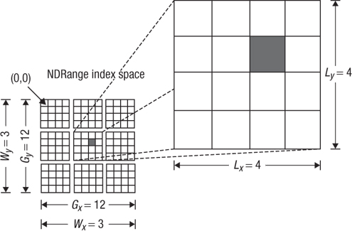
In Figure 1.7 we provide a concrete example where each small square is a work-item. For this example, we use the default offset of zero in each dimension. Study this figure and make sure that you understand that the shaded square with global index (6, 5) falls in the work-group with ID (1, 1) and local index (2, 1).

Figure 1.7 An example of how the global IDs, local IDs, and work-group indices are related for a two-dimensional NDRange. Other parameters of the index space are defined in the figure. The shaded block has a global ID of (g_x, g_y) = (6, 5) and a work-group plus local ID of (w_x, w_y) = (1, 1) and (l_x, l_y) =(2, 1).

If all of these index manipulations seem confusing, don’t worry. In many cases OpenCL programmers just work in the global index space. Over time, as you work with OpenCL and gain experience working with the different types of indices, these sorts of manipulations will become second nature to you.

The OpenCL execution model is quite flexible. This model supports a wide range of programming models. In designing OpenCL, however, only two models were explicitly considered: data parallelism and task parallelism. We will return to these models and their implications for OpenCL later. But first, we need to complete our tour of the OpenCL execution model.

Context

The computational work of an OpenCL application takes place on the OpenCL devices. The host, however, plays a very important role in the OpenCL application. It is on the host where the kernels are defined. The host establishes the context for the kernels. The host defines the NDRange and the queues that control the details of how and when the kernels execute. All of these important functions are contained in the APIs within OpenCL’s definition.

The first task for the host is to define the context for the OpenCL application. As the name implies, the context defines the environment within which the kernels are defined and execute. To be more precise, we define the context in terms of the following resources:

• Devices: the collection of OpenCL devices to be used by the host

• Kernels: the OpenCL functions that run on OpenCL devices

• Program objects: the program source code and executables that implement the kernels

• Memory objects: a set of objects in memory that are visible to OpenCL devices and contain values that can be operated on by instances of a kernel

The context is created and manipulated by the host using functions from the OpenCL API. For example, consider the heterogeneous platform from Figure 1.3. This system has two multicore CPUs and a GPU. The host program is running on one of the CPUs. The host program will query the system to discover these resources and then decide which devices to use in the OpenCL application. Depending on the problem and the kernels to be run, the host may choose the GPU, the other CPU, other cores on the same CPU, or any combination of these. Once made, this choice defines the OpenCL devices within the current context.

Also included in the context are one or more program objects that contain the code for the kernels. The choice of the name program object is a bit confusing. It is better to think of these as a dynamic library from which the functions used by the kernels are pulled. The program object is built at runtime within the host program. This might seem strange to programmers from outside the graphics community. Consider for a moment the challenge faced by an OpenCL programmer. He or she writes the OpenCL application and passes it to the end user, but that user could choose to run the application anywhere. The application programmer has no control over which GPUs or CPUs or other chips the end user may run the application on. All the OpenCL programmer knows is that the target platform will be conformant to the OpenCL specification.

The solution to this problem is for the program object to be built from source at runtime. The host program defines the devices within the context. Only at that point is it possible to know how to compile the program source code to create the code for the kernels. As for the source code itself, OpenCL is quite flexible about the form. In many cases, it is a regular string either statically defined in the host program, loaded from a file at runtime, or dynamically generated inside the host program.

Our context now includes OpenCL devices and a program object from which the kernels are pulled for execution. Next we consider how the kernels interact with memory. The detailed memory model used by OpenCL will be described later. For the sake of our discussion of the context, we need to understand how the OpenCL memory works only at a high level. The crux of the matter is that on a heterogeneous platform, there are often multiple address spaces to manage. The host has the familiar address space expected on a CPU platform, but the devices may have a range of different memory architectures. To deal with this situation, OpenCL introduces the idea of memory objects. These are explicitly defined on the host and explicitly moved between the host and the OpenCL devices. This does put an extra burden on the programmer, but it lets us support a much wider range of platforms.

We now understand the context within an OpenCL application. The context is the OpenCL devices, program objects, kernels, and memory objects that a kernel uses when it executes. Now we can move on to how the host program issues commands to the OpenCL devices.

Command-Queues

The interaction between the host and the OpenCL devices occurs through commands posted by the host to the command-queue. These commands wait in the command-queue until they execute on the OpenCL device. A command-queue is created by the host and attached to a single OpenCL device after the context has been defined. The host places commands into the command-queue, and the commands are then scheduled for execution on the associated device. OpenCL supports three types of commands:

• Kernel execution commands execute a kernel on the processing elements of an OpenCL device.

• Memory commands transfer data between the host and different memory objects, move data between memory objects, or map and unmap memory objects from the host address space.

• Synchronization commands put constraints on the order in which commands execute.

In a typical host program, the programmer defines the context and the command-queues, defines memory and program objects, and builds any data structures needed on the host to support the application. Then the focus shifts to the command-queue. Memory objects are moved from the host onto the devices; kernel arguments are attached to memory objects and then submitted to the command-queue for execution. When the kernel has completed its work, memory objects produced in the computation may be copied back onto the host.

When multiple kernels are submitted to the queue, they may need to interact. For example, one set of kernels may generate memory objects that a following set of kernels needs to manipulate. In this case, synchronization commands can be used to force the first set of kernels to complete before the following set begins.

There are many additional subtleties associated with how the commands work in OpenCL. We will leave those details for later in the book. Our goal now is just to understand the command-queues and hence gain a high-level understanding of OpenCL commands.

So far, we have said very little about the order in which commands execute or how their execution relates to the execution of the host program. The commands always execute asynchronously to the host program. The host program submits commands to the command-queue and then continues without waiting for commands to finish. If it is necessary for the host to wait on a command, this can be explicitly established with a synchronization command.

Commands within a single queue execute relative to each other in one of two modes:

• In-order execution: Commands are launched in the order in which they appear in the command-queue and complete in order. In other words, a prior command on the queue completes before the following command begins. This serializes the execution order of commands in a queue.

• Out-of-order execution: Commands are issued in order but do not wait to complete before the following commands execute. Any order constraints are enforced by the programmer through explicit synchronization mechanisms.

All OpenCL platforms support the in-order mode, but the out-of-order mode is optional. Why would you want to use the out-of-order mode? Consider Figure 1.5, where we introduced the concept of load balancing. An application is not done until all of the kernels complete. Hence, for an efficient program that minimizes the runtime, you want all compute units to be fully engaged and to run for approximately the same amount of time. You can often do this by carefully thinking about the order in which you submit commands to the queues so that the in-order execution achieves a well-balanced load. But when you have a set of commands that take different amounts of time to execute, balancing the load so that all compute units stay fully engaged and finish at the same time can be difficult. An out-of-order queue can take care of this for you. Commands can execute in any order, so if a compute unit finishes its work early, it can immediately fetch a new command from the command-queue and start executing a new kernel. This is called automatic load balancing, and it is a well-known technique used in the design of parallel algorithms driven by command-queues (see the Master-Worker pattern in T. G. Mattson et al., Patterns for Parallel Programming⁵).

Anytime you have multiple executions occurring inside an application, the potential for disaster exists. Data may be accidentally used before it has been written, or kernels may execute in an order that leads to wrong answers. The programmer needs some way to manage any constraints on the commands. We’ve hinted at one, a synchronization command to tell a set of kernels to wait until an earlier set finishes. This is often quite effective, but there are times when more sophisticated synchronization protocols are needed.

To support custom synchronization protocols, commands submitted to the command-queue generate event objects. A command can be told to wait until certain conditions on the event objects exist. These events can also be used to coordinate execution between the host and the OpenCL devices. We’ll say more about these events later.

Finally, it is possible to associate multiple queues with a single context for any of the OpenCL devices within that context. These two queues run concurrently and independently with no explicit mechanisms within OpenCL to synchronize between them.

Memory Model

The execution model tells us how the kernels execute, how they interact with the host, and how they interact with other kernels. To describe this model and the associated command-queue, we made a brief mention of memory objects. We did not, however, define the details of these objects, neither the types of memory objects nor the rules for how to safely use them. These issues are covered by the OpenCL memory model.

OpenCL defines two types of memory objects: buffer objects and image objects. A buffer object, as the name implies, is just a contiguous block of memory made available to the kernels. A programmer can map data structures onto this buffer and access the buffer through pointers. This provides flexibility to define just about any data structure the programmer wishes (subject to limitations of the OpenCL kernel programming language).

Image objects, on the other hand, are restricted to holding images. An image storage format may be optimized to the needs of a specific OpenCL device. Therefore, it is important that OpenCL give an implementation the freedom to customize the image format. The image memory object, therefore, is an opaque object. The OpenCL framework provides functions to manipulate images, but other than these specific functions, the contents of an image object are hidden from the kernel program.

OpenCL also allows a programmer to specify subregions of memory objects as distinct memory objects (added with the OpenCL 1.1 specification). This makes a subregion of a large memory object a first-class object in OpenCL that can be manipulated and coordinated through the command-queue.

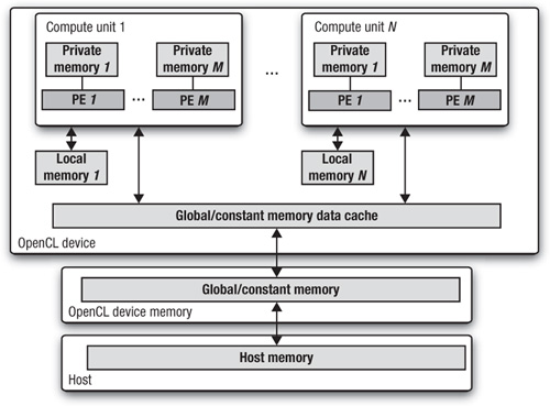
Understanding the memory objects themselves is just a first step. We also need to understand the specific abstractions that govern their use in an OpenCL program. The OpenCL memory model defines five distinct memory regions:

• Host memory: This memory region is visible only to the host. As with most details concerning the host, OpenCL defines only how the host memory interacts with OpenCL objects and constructs.

• Global memory: This memory region permits read/write access to all work-items in all work-groups. Work-items can read from or write to any element of a memory object in global memory. Reads and writes to global memory may be cached depending on the capabilities of the device.

• Constant memory: This memory region of global memory remains constant during the execution of a kernel. The host allocates and initializes memory objects placed into constant memory. Work-items have read-only access to these objects.

• Local memory: This memory region is local to a work-group. This memory region can be used to allocate variables that are shared by all work-items in that work-group. It may be implemented as dedicated regions of memory on the OpenCL device. Alternatively, the local memory region may be mapped onto sections of the global memory.

• Private memory: This region of memory is private to a work-item. Variables defined in one work-item’s private memory are not visible to other work-items.

The memory regions and how they relate to the platform and execution models are described in Figure 1.8. The work-items run on PEs and have their own private memory. A work-group runs on a compute unit and shares a local memory region with the work-items in the group. The OpenCL device memory works with the host to support global memory.

Figure 1.8 A summary of the memory model in OpenCL and how the different memory regions interact with the platform model

The host and OpenCL device memory models are, for the most part, independent of each other. This is by necessity, given that the host is defined outside of OpenCL. They do, however, at times need to interact. This interaction occurs in one of two ways: by explicitly copying data or by mapping and unmapping regions of a memory object.

To copy data explicitly, the host enqueues commands to transfer data between the memory object and host memory. These memory transfer commands may be blocking or non-blocking. The OpenCL function call for a blocking memory transfer returns once the associated memory resources on the host can be safely reused. For a non-blocking memory transfer, the OpenCL function call returns as soon as the command is enqueued regardless of whether host memory is safe to use.

The mapping/unmapping method of interaction between the host and OpenCL memory objects allows the host to map a region from the memory object into its own address space. The memory map command (which is enqueued on the command-queue like any other OpenCL command) may be blocking or non-blocking. Once a region from the memory object has been mapped, the host can read or write to this region. The host unmaps the region when accesses (reads and/or writes) to this mapped region by the host are complete.

When concurrent execution is involved, however, the memory model needs to carefully define how memory objects interact in time with the kernel and host. This is the problem of memory consistency. It is not enough to say where the memory values will go. You also must define when these values are visible across the platform.

Once again, OpenCL doesn’t stipulate the memory consistency model on the host. Let’s start with the memory farthest from the host (private memory region) and work toward the host. Private memory is not visible to the host. It is visible only to an individual work-item. This memory follows the load/store memory model familiar to sequential programming. In other words, the loads and stores into private memory cannot be reordered to appear in any order other than that defined in the program text.

For the local memory, the values seen by a set of work-items within a work-group are guaranteed to be consistent at work-group synchronization points. For example, a work-group barrier requires that all loads and stores defined before the barrier complete before any work-items in the group proceed past the barrier. In other words, the barrier marks a point in the execution of the set of work-items where the memory is guaranteed to be in a consistent and known state before the execution continues.

Because local memory is shared only within a work-group, this is sufficient to define the memory consistency for local memory regions. For the work-items within a group, the global memory is also made consistent at a work-group barrier. Even though this memory is shared between work-groups, however, there is no way to enforce consistency of global memory between the different work-groups executing a kernel.

For the memory objects, OpenCL defines a relaxed consistency model. In other words, the values seen in memory by an individual work-item are not guaranteed to be consistent across the full set of work-items at all times. At any given moment, the loads and stores into OpenCL memory objects may appear to occur in a different order for different work-items. This is called a relaxed consistency model because it is less strict than the load/store model one would expect if the concurrent execution were to exactly match the order from a serial execution.

The last step is to define the consistency of memory objects relative to the commands on the command-queue. In this case, we use a modified version of release consistency. When all the work-items associated with a kernel complete, loads and stores for the memory objects released by this kernel are completed before the kernel command is signaled as finished. For the in-order queue, this is sufficient to define the memory consistency between kernels. For an out-of-order queue there are two options (called synchronization points). The first is for consistency to be forced at specific synchronization points such as a command-queue barrier. The other option is for consistency to be explicitly managed through the event mechanisms we’ll describe later. These same options are used to enforce consistency between the host and the OpenCL devices; that is, memory is consistent only at synchronization points on the command-queue.

Programming Models

The OpenCL execution model defines how an OpenCL application maps onto processing elements, memory regions, and the host. It is a “hardware-centric” model. We now shift gears and describe how we map parallel algorithms onto OpenCL using a programming model. Programming models are intimately connected to how programmers reason about their algorithms. Hence, the nature of these models is more flexible than that of the precisely defined execution model.

OpenCL was defined with two different programming models in mind: task parallelism and data parallelism. As you will see, you can even think in terms of a hybrid model: tasks that contain data parallelism. Programmers are very creative, and we can expect over time that additional programming models will be created that will map onto OpenCL’s basic execution model.

Data-Parallel Programming Model

We described the basic idea of a data-parallel programming model earlier (see Figure 1.4). Problems well suited to the data-parallel programming model are organized around data structures, the elements of which can be updated concurrently. In essence, a single logical sequence of instructions is applied concurrently to the elements of the data structure. The structure of the parallel algorithm is designed as a sequence of concurrent updates to the data structures within a problem.

This programming model is a natural fit with OpenCL’s execution model. The key is the NDRange defined when a kernel is launched. The algorithm designer aligns the data structures in his or her problem with the NDRange index space and maps them onto OpenCL memory objects. The kernel defines the sequence of instructions to be applied concurrently as the work-items in an OpenCL computation.

In more complicated data-parallel problems, the work-items in a single work-group may need to share data. This is supported through data stored in the local memory region. Anytime dependencies are introduced between work-items, care must be taken that regardless of the order in which the work-items complete, the same results are produced. In other words, the work-items may need to synchronize their execution. Work-items in a single work-group can participate in a work-group barrier. As we stated earlier, all the work-items within a work-group must execute the barrier before any are allowed to continue execution beyond the barrier. Note that the work-group barrier must be encountered by all work-items of a work-group executing the kernel or by none at all.

OpenCL 1.1 doesn’t provide any mechanism for synchronization between work-items from different work-groups while executing a kernel. This is an important limitation for programmers to keep in mind when designing parallel algorithms.

As an example of when work-items need to share information, consider a set of work-items participating in some sort of reduction. A reduction is when a collection of data elements is reduced to a single element by some type of associative operation. The most common examples are summation or finding extreme values (max or min) of a set of data elements. In a reduction, the work-items carry out a computation to produce the data elements that will be reduced. This must complete on all work-items before a subset of the work-items (often a subset of size one) does the accumulation for all the work-items.

OpenCL provides hierarchical data parallelism: data parallelism from work-items within a work-group plus data parallelism at the level of work-groups. The OpenCL specification discusses two variants of this form of data parallelism. In the explicit model, the programmer takes responsibility for explicitly defining the sizes of the work-groups. With the second model, the implicit model, the programmer just defines the NDRange space and leaves it to the system to choose the work-groups.

If the kernel doesn’t contain any branch statements, each work-item will execute identical operations but on a subset of data items selected by its global ID. This case defines an important subset of the data-parallel model known as Single Instruction Multiple Data or SIMD. Branch statements within a kernel, however, can lead each work-item to execute very different operations. While each work-item is using the same “program” (i.e., the kernel), the actual work it accomplishes can be quite different. This is often known as a Single Program Multiple Data or SPMD model (see the SPMD pattern in Mattson’s Patterns for Parallel Programming).

OpenCL supports both SIMD and SPMD models. On platforms with restricted bandwidth to instruction memory or if the processing elements map onto a vector unit, the SIMD model can be dramatically more efficient. Hence, it is valuable for a programmer to understand both models and know when to use one or the other.

There is one case when an OpenCL program is strictly SIMD: the vector instructions defined in Chapter 4, “Programming with OpenCL C.” These instructions let you explicitly issue instructions for vector units attached to a processing element. For example, the following instructions come from a numerical integration program (the integrand is 4.0/(1 + x²)). In this program, we unroll the integration loop eightfold and compute eight steps in the integration at once using the native vector instructions on the target platform.

float8 x, psum_vec;
float8 ramp= (float8)(0.5, 1.5, 2.5, 3.5,
                      4.5, 5.5, 6.5, 7.5};
float8 four= (float8)(4.0);  // fill with 8 4's
float8 one = (float8)(1.0);  // fill with 8 1's
float  step_number; // step number from loop index
float  step_size;   // Input integration step size

. . . and later inside a loop body . . .

    x = ((float8)step_number +ramp)*step_size;
    psum_vec+=four/(one + x*x);

Given the wide range of vector instruction sets on the market, having a portable notation for explicit vector instructions is an extremely convenient feature within OpenCL.

In closing, data parallelism is a natural fit to the OpenCL execution model items. The model is hierarchical because a data-parallel computation (the work-items) may include vector instructions (SIMD) and be part of larger block-level data parallelism (work-groups). All of these work together to create a rich environment for expressing data-parallel algorithms.

Task-Parallel Programming Model

The OpenCL execution model was clearly designed with data parallelism as a primary target. But the model also supports a rich array of task-parallel algorithms.

OpenCL defines a task as a kernel that executes as a single work-item regardless of the NDRange used by other kernels in the OpenCL application. This is used when the concurrency a programmer wishes to exploit is internal to the task. For example, the parallelism may be expressed solely in terms of vector operations over vector types. Or perhaps the task uses a kernel defined with the native kernel interface and the parallelism is expressed using a programming environment outside of OpenCL.

A second version of task parallelism appears when kernels are submitted as tasks that execute at the same time with an out-of-order queue. For example, consider the collection of independent tasks represented schematically in Figure 1.5. On a quad-core CPU, one core could be the host and the other three cores configured as compute units within an OpenCL device. The OpenCL application could enqueue all six tasks and leave it to the compute units to dynamically schedule the work. When the number of tasks is much greater than the number of compute units, this strategy can be a very effective way to produce a well-balanced load. This style of task parallelism, however, will not work on all OpenCL platforms because the out-of-order mode for a command-queue is an optional feature in OpenCL 1.1.

A third version of task parallelism occurs when the tasks are connected into a task graph using OpenCL’s event model. Commands submitted to an event queue may optionally generate events. Subsequent commands can wait for these events before executing. When combined with a command-queue that supports the out-of-order execution model, this lets the OpenCL programmer define static task graphs in OpenCL, with the nodes in the graph being tasks and the edges dependencies between the nodes (managed by events). We will discuss this topic in great detail in Chapter 9, “Events.”

Parallel Algorithm Limitations

The OpenCL framework defines a powerful foundation for data-parallel and task-parallel programming models. A wide range of parallel algorithms can map onto these models, but there are restrictions. Because of the wide range of devices that OpenCL supports, there are limitations to the OpenCL execution model. In other words, the extreme portability of OpenCL comes at a cost of generality in the algorithms we can support.

The crux of the matter comes down to the assumptions made in the execution model. When we submit a command to execute a kernel, we can only assume that the work-items in a group will execute concurrently. The implementation is free to run individual work-groups in any order—including serially (i.e., one after the other). This is also the case for kernel executions. Even when the out-of-order queue mode is enabled, a conforming implementation is free to serialize the execution of the kernels.

These constraints on how concurrency is expressed in OpenCL limit the way data can be shared between work-groups and between kernels. There are two cases you need to understand. First, consider the collection of work-groups associated with a single kernel execution. A conforming implementation of OpenCL can order these any way it chooses. Hence, we cannot safely construct algorithms that depend on the details of how data is shared between the work-groups servicing a single kernel execution.

Second, consider the order of execution for multiple kernels. They are submitted for execution in the order in which they are enqueued, but they execute serially (in-order command-queue mode) or concurrently (out-of-order command-queue mode). However, even with the out-of-order queue an implementation is free to execute kernels in serial order. Hence, early kernels waiting on events from later kernels can deadlock. Furthermore, the task graphs associated with an algorithm can only have edges that are unidirectional and point from nodes enqueued earlier in the command-queue to kernels enqueued later in the command-queue.

These are serious limitations. They mean that there are parallel design patterns that just can’t be expressed in OpenCL. Over time, however, as hardware evolves and, in particular, GPUs continue to add features to support more general-purpose computing, we will fix these limitations in future releases of OpenCL. For now, we just have to live with them.

Other Programming Models

A programmer is free to combine OpenCL’s programming models to create a range of hybrid programming models. We’ve already mentioned the case where the work-items in a data-parallel algorithm contain SIMD parallelism through the vector instructions.

As OpenCL implementations mature, however, and the out-of-order mode on command-queues becomes the norm, we can imagine static task graphs where each node is a data-parallel algorithm (multiple work-items) that includes SIMD vector instructions.

OpenCL exposes the hardware through a portable platform model and a powerful execution model. These work together to define a flexible hardware abstraction layer. Computer scientists are free to layer other programming models on top of the OpenCL hardware abstraction layer. OpenCL is young and we can’t cite any concrete examples of programming models from outside OpenCL’s specification running on OpenCL platforms. But stay tuned and watch the literature. It’s only a matter of time until this happens.

OpenCL and Graphics

OpenCL was created as a response to GPGPU programming. People had GPUs for graphics and started using them for the non-graphics parts of their workloads. And with that trend, heterogeneous computing (which has been around for a very long time) collided with graphics, and the need for an industry standard emerged.

OpenCL has stayed close to its graphics roots. OpenCL is part of the Khronos family of standards, which includes the graphics standards OpenGL (www.khronos.org/opengl/) and OpenGL ES (www.khronos.org/opengles/). Given the importance of the operating systems from Microsoft, OpenCL also closely tracks developments in DirectX (www.gamesforwindows.com/en-US/directx/).

To start our discussion of OpenCL and graphics we return to the image memory objects we mentioned earlier. Image memory objects are one-, two-, or three-dimensional objects that hold textures, frame buffers, or images. An implementation is free to support a range of image formats, but at a minimum, it must support the standard RGBA format. The image objects are manipulated using a set of functions defined within OpenCL. OpenCL also defines sampler objects so that programmers can sample and filter images. These features are integrated into the core set of image manipulation functions in the OpenCL APIs.

Once images have been created, they must pass to the graphics pipeline to be rendered. Hence including an interface to the standard graphics APIs would be useful within OpenCL. Not every vendor working on OpenCL, however, is interested in these graphics standards. Therefore, rather than include this in the core OpenCL specification, we define these as a number of optional extensions in the appendices to the OpenCL standard. These extensions include the following functionalities:

• Creating an OpenCL context from an OpenGL context

• Sharing memory objects between OpenCL, OpenGL, and OpenGL ES

• Creating OpenCL event objects from OpenGL sync objects

• Sharing memory objects with Direct3D version 10

These will be discussed later in the book.

The Contents of OpenCL

So far we have focused on the ideas behind OpenCL. Now we shift gears and talk about how these ideas are supported within the OpenCL framework. The OpenCL framework is divided into the following components:

• OpenCL platform API: The platform API defines functions used by the host program to discover OpenCL devices and their capabilities as well as to create the context for the OpenCL application.

• OpenCL runtime API: This API manipulates the context to create command-queues and other operations that occur at runtime. For example, the functions to submit commands to the command-queue come from the OpenCL runtime API.

• The OpenCL programming language: This is the programming language used to write the code for kernels. It is based on an extended subset of the ISO C99 standard and hence is often referred to as the OpenCL C programming language.

In the next few subsections we will provide a high-level overview of each of these components. Details will be left for later in the book, but it will be helpful as you start working with OpenCL to understand what’s happening at a high level.

Platform API

The term platform has a very specific meaning in OpenCL. It refers to a particular combination of the host, the OpenCL devices, and the OpenCL framework. Multiple OpenCL platforms can exist on a single heterogeneous computer at one time. For example, the CPU vendor and the GPU vendor may define their own OpenCL frameworks on a single system. Programmers need a way to query the system about the available OpenCL frameworks. They need to find out which OpenCL devices are available and what their characteristics are. And they need to control which subset of these frameworks and devices will constitute the platform used in any given OpenCL application.

This functionality is addressed by the functions within OpenCL’s platform API. As you will see in later chapters when we focus on the code OpenCL programmers write for the host program, every OpenCL application opens in a similar way, calling functions from the platform API to ultimately define the context for the OpenCL computation.

Runtime API

The functions in the platform API ultimately define the context for an OpenCL application. The runtime API focuses on functions that use this context to service the needs of an application. This is a large and admittedly complex collection of functions.

The first job of the runtime API is to set up the command-queues. You can attach a command-queue to a single device, but multiple command-queues can be active at one time within a single context.

With the command-queues in place, the runtime API is used to define memory objects and any objects required to manipulate them (such as sampler objects for image objects). Managing memory objects is an important task. To support garbage collection, OpenCL keeps track of how many instances of kernels use these objects (i.e., retain a memory object) and when kernels are finished with a memory object (i.e., release a memory object).

Another task managed by the runtime API is to create the program objects used to build the dynamic libraries from which kernels are defined. The program objects, the compiler to compile them, and the definition of the kernels are all handled in the runtime layer.

Finally, the commands that interact with the command-queue are all issued by functions from the runtime layer. Synchronization points for managing data sharing and to enforce constraints on the execution of kernels are also handled by the runtime API.

As you can see, functions from the runtime API do most of the heavy lifting for the host program. To attempt to master the runtime API in one stretch, starting from the beginning and working through all the functions, is overwhelming. We have found that it is much better to use a pragmatic approach. Master the functions you actually use. Over time you will cover and hence master them all, but you will learn them in blocks driven by the specific needs of an OpenCL application.

Kernel Programming Language

The host program is very important, but it is the kernels that do the real work in OpenCL. Some OpenCL implementations let you interface to native kernels written outside of OpenCL, but in most cases you will need to write kernels to carry out the specific work in your application.

The kernel programming language in OpenCL is called the OpenCL C programming language because we anticipate over time that we may choose to define other languages within the specification. It is derived from the ISO C99 language.

In OpenCL, we take great care to support portability. This forces us to standardize around the least common dominator between classes of OpenCL devices. Because there are features in C99 that only CPUs can support, we had to leave out some of the language features in C99 when we defined the OpenCL C programming language. The major language features we deleted include

• Recursive functions

• Pointers to functions

• Bit fields

In addition, we cannot support the full set of standard libraries. The list of standard headers not allowed in the OpenCL programming language is long, but the ones programmers will probably miss the most are stdio.h and stdlib.h. Once again, these libraries are hard to support once you move away from a general-purpose processor as the OpenCL device.

Other restrictions arise from the need to maintain fidelity to OpenCL’s core abstractions. For example, OpenCL defines a range of memory address spaces. A union or structure cannot mix these types. Also, there are types defined in OpenCL that are opaque, for example, the memory objects that support images. The OpenCL C programming language prevents one from doing anything with these types other than passing them as arguments to functions.

We restricted the OpenCL C programming language to match the needs of the key OpenCL devices used with OpenCL. This same motivation led us to extend the languages as well as

• Vector types and operations on instances of those types

• Address space qualifiers to support control over the multiple address spaces in OpenCL

• A large set of built-in functions to support functionality commonly needed in OpenCL applications

• Atomic functions for unsigned integer and single-precision scalar variables in global and local memory

Most programming languages ignore the specifics of the floating-point arithmetic system. They import the arithmetic system from the hardware and avoid the topic altogether. Because all major CPUs support the IEEE 754 and 854 standards, this strategy has worked. In essence, by converging around these floating-point standards, the hardware vendors took care of the floating-point definition for the language vendors.

In the heterogeneous world, however, as you move away from the CPU, the support for floating-point arithmetic is more selective. Working closely with the hardware vendors, we wanted to create momentum that would move them over time to complete support for the IEEE floating-point standards. At the same time, we didn’t want to be too hard on these vendors, so we gave them flexibility to avoid some of the less used but challenging-to-implement features of the IEEE standards. We will discuss the details later, but at a high level OpenCL requires the following:

• Full support for the IEEE 754 formats. Double precision is optional, but if it is provided, it must follow the IEEE 754 formats as well.

• The default IEEE 754 rounding mode of “round to nearest.” The other rounding modes, while highly encouraged (because numerical analysts need them), are optional.

• Rounding modes in OpenCL are set statically, even though the IEEE specifications require dynamic variation of rounding modes.

• The special values of INF (infinity) and NaN (Not a Number) must be supported. The signaling NaN (always a problem in concurrent systems) is not required.

• Denormalized numbers (numbers smaller than one times the largest supported negative exponent) can be flushed to zero. If you don’t understand why this is significant, you are in good company. This is another feature that numerical analysts depend on but few programmers understand.

There are a few additional rules pertaining to floating-point exceptions, but they are too detailed for most people and too obscure to bother with at this time. The point is that we tried very hard to require the bulk of IEEE 754 while leaving off some of the features that are more rarely used and difficult to support (on a heterogeneous platform with vector units).

The OpenCL specification didn’t stop with the IEEE standards. In the OpenCL specification, there are tables that carefully define the allowed relative errors in math functions. Getting all of these right was an ambitious undertaking, but for the programmers who write detailed numerical code, having these defined is essential.

When you put these floating-point requirements, restrictions, and extensions together, you have a programming language well suited to the capabilities of current heterogeneous platforms. And as the processors used in these platforms evolve and become more general, the OpenCL C programming language will evolve as well.

OpenCL Summary

We have now covered the basic components of the core OpenCL framework. It is important to understand them in isolation (as we have largely presented them). To pull this together to create a complete picture of OpenCL, we provide a summary of the basic workflow of an application as it works through the OpenCL framework, shown in Figure 1.9.

Figure 1.9 This block diagram summarizes the components of OpenCL and the actions that occur on the host during an OpenCL application.

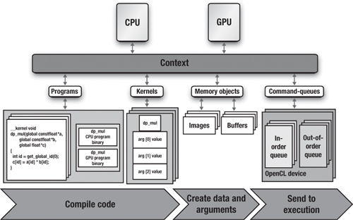
You start with a host program that defines the context. The context in Figure 1.9 contains two OpenCL devices, a CPU and a GPU. Next we define the command-queues. In this case we have two queues, an in-order command-queue for the GPU and an out-of-order command-queue for the CPU. The host program then defines a program object that is compiled to generate kernels for both OpenCL devices (the CPU and the GPU). Next the host program defines any memory objects required by the program and maps them onto the arguments of the kernels. Finally, the host program enqueues commands to the command-queues to execute the kernels.

The Embedded Profile

OpenCL programs address the needs of a tremendous range of hardware platforms. From HPC Servers to laptops to cell phones, OpenCL has a tremendous reach. For most of the standard, this range is not a problem. For a few features, however, the embedded processors just can’t match the requirements in the standard.

We had two choices: take the easy route and leave it to each vendor to decide how to relax the OpenCL specification to meet their needs, or do the hard work ourselves and define exactly how to change OpenCL for embedded processors. We chose the harder approach; that is, we defined how the OpenCL specification should be changed to fit the needs of embedded processors. We describe the embedded profile in Chapter 13, “OpenCL Embedded Profile.”

We did not want to create a whole new standard, however. To do so would put us in the awkward position of struggling to keep the two standards from diverging. Hence, the final section of the OpenCL specification defines the “embedded profile,” which we describe later in the book. Basically, we relaxed the floating-point standards and some of the larger data types because these are not often required in the embedded market. Some of the image requirements (such as the 3D image format) were also relaxed. Atomic functions are not required, and the relative errors of built-in math functions were relaxed. Finally, some of the minimum parameters for properties of different components of the framework (such as the minimum required size of the private memory region) were reduced to match the tighter memory size constraints used in the embedded market.

As you can see, for the most part, OpenCL for embedded processors is very close to the full OpenCL definition. Most programmers will not even notice these differences.

Learning OpenCL

OpenCL is an industry standard for writing parallel programs to execute on heterogeneous platforms. These platforms are here today and, as we hope we have shown you, will be the dominant architecture for computing into the foreseeable future. Hence, programmers need to understand heterogeneous platforms and become comfortable programming for them.

In this chapter we have provided a conceptual framework to help you understand OpenCL. The platform model defines an abstraction that applies to the full diversity of heterogeneous systems. The execution model within OpenCL describes whole classes of computations and how they map onto the platform model. The framework concludes with programming models and a memory model, which together give the programmer the tools required to reason about how software elements in an OpenCL program interact to produce correct results.

Equipped with this largely theoretical knowledge, you can now start to learn how to use the contents of OpenCL. We begin with the following chapter, where we will write our first OpenCL program.