
Chapter 22. Sparse Matrix-Vector Multiplication
By Gordon Fossum
This chapter describes an optimized implementation of the Sparse Matrix-Vector Multiplication (SpMV) algorithm using OpenCL.
Sparse matrices, for the purposes of this chapter, are defined as large two-dimensional matrices in which the vast majority of the elements of the matrix are equal to zero. They may be largely diagonal, or not. They may be symmetric, or not (perhaps not even square). They may be singular (containing entire rows with no non-zero elements), or not. They are used to characterize and solve problems in a wide variety of domains.
The sample uses a new portable tiled and packetized sparse matrix data format, which has both a single-precision and a double-precision instantiation. The format is intended to improve cache utilization and minimize “gather/scatter” inefficiency.
The implementation demonstrates OpenCL’s ability to bridge the gap between hardware-specific code (fast, but not portable) and single-source code (very portable, but slow), yielding a high-performance, efficient implementation on a variety of hardware that is almost as fast as a hardware-specific implementation.
These results are accomplished with kernels written in OpenCL C that can be compiled and run on any conforming OpenCL platform.
Sparse Matrix-Vector Multiplication (SpMV) Algorithm
The SpMV algorithm efficiently multiplies a sparse matrix by an input vector, producing an output vector. That is, it computes an equation of the form y = A * x, where y and x are vectors and A is a matrix, which in this case is a sparse matrix.
Various sparse matrix representation schemes have been proposed that seek to balance the competing needs of minimizing the memory footprint of the sparse matrix while maximizing the performance of the algorithm.
One traditional method for representing a sparse matrix is to create three arrays of binary data, one containing the non-zero floating-point data of the matrix (referred to as Val); another, same-size array containing the column index where each of these non-zero elements comes from (referred to as Col_ind); and a third, smaller array containing the indices into the previous two arrays where each row starts (referred to as Row_ptr). This is commonly referred to as either the compressed sparse row (CSR) or compressed row storage (CRS) format.
For example, look at the sparse matrix in Figure 22.1.
Figure 22.1 Sparse matrix example
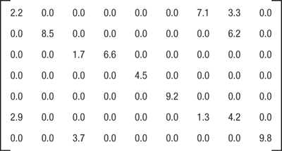
This sparse matrix would be represented with three arrays, as follows:
Val = {2.2, 7.1, 3.3, 8.5, 6.2, 1.7, 6.6, 4.5, 9.2, 2.9, 1.3, 4.2, 3.7, 9.8};
Col_ind = {0, 6, 7, 1, 7, 2, 3, 4, 5, 0, 6, 7, 2, 8};
Row_ptr = {0, 3, 5, 7, 8, 9, 12};
A more basic method is to create an ASCII file with header information consisting of the name of the matrix, whether the matrix is symmetric or not (symmetric or general, respectively), and whether the file merely contains the pattern of non-zero content or actually contains the values of these non-zero elements (pattern or coordinate, respectively). The body of this file then contains a series of lines, where each line contains a row index, a column index, and (optionally) a data value. This is referred to as Matrix Market (MM) exchange format (see http://math.nist.gov/MatrixMarket/formats.html for more information) and is used most notably by the University of Florida in its large collection of sparse and dense matrices (www.cise.ufl.edu/research/sparse/matrices).
Various other matrix representations are described in previous implementations of SpMV, which were targeted at particular hardware platforms and developed before the advent of OpenCL.
In the paper “Efficient Sparse Matrix-Vector Multiplication on CUDA,”1 a hybrid approach is adopted that seeks to optimize for several potential storage formats: coordinate (COO), CSR, ELLPACK, and a Packet format, which differs from the one in this chapter in several particulars. The two most important are that the output indices are not individually stored, but rather a single offset is loaded into the packet, and all output data is implicitly keyed off of that one offset. Further, every read-modify-write operation to the local output buffer is fully coalesced across 16 compute units.
In the paper “Optimizing Sparse Matrix-Vector Multiplication on GPUs,”2 the authors choose to concentrate on the CSR format and implement variants on CSR that are more suited for GPU architectures. In particular, 16 threads are assigned to each row in the CSR format, and each thread strides through the row, computing on only every sixteenth element. The format is further modified to pad the rows to multiples of 16. Further, they analyze the matrix to identify dense sub-blocks and deal with them in a special way.
The device-independent tiled and packetized sparse matrix representation used by this implementation has a single format (actually a format for single precision and a format for double precision) and achieves perfect coalescing of all matrix accesses and output accesses.
Description of This Implementation
This implementation has a single source file of host code, which performs the following operations:
• Reads the Matrix Market format matrix data from disk
• Initializes the OpenCL environment
• Creates the tiled and packetized matrix
• Initializes the input vector
• Calls the kernel code passing it the input vector, the matrix, and the output vector
• Verifies the results
• Reports performance data
• Shuts down the OpenCL environment and cleans up
It further provides a single source file of kernel code, containing two similar kernels. These two kernels accommodate two different methods of hiding memory latency, one implicit (using multithreading or cache hierarchies) and the other one explicit (double buffering with asynchronous DMAs).
The first (implicit) kernel implements read/write direct access to global memory serially with the computations on that data. This kernel is best used on an OpenCL CPU or GPU device.
As previously mentioned, this kernel is run in parallel on a large number of compute devices or compute units, in batches of local work-groups. Within each local work-group, we explicitly acknowledge and use a smaller computational grouping, which we call a team of processing elements that executes on a compute unit, which has a size of 16 for a GPU and a size of 1 for a CPU. The use of a team size of 1 on CPUs derives from a need to avoid current inefficiencies in OpenCL compilers, wherein multiple work-groups are simulated with a loop-unrolling mechanism that unfortunately results in cache-thrashing behavior on many CPUs. When future compilers are available that unroll their loops in a more efficient fashion, all teams on all devices will have a size of 16. Within the GPU device, the local work-group is composed of one or more of these teams. Thus, the team size is 16, and the local work-group size might be 64 or 128, for example. There are several reasons why 16 is the best size to use:
• Every GPU we have encountered has a natural affinity for grouping its global memory read-write operations in multiples of 64 bytes (or 16 4-byte elements).
• A group of 16 single-precision elements, along with their necessary control and index information, conveniently fits into a 128-byte cache line.
• GPUs enjoy improved performance when the algorithm can perform coalesced memory accesses, which are grouped in multiples of 16.
An if test within this first kernel is used to distinguish between GPUs (team size 16) and CPUs (team size 1). The GPU clause computes a single product, and the CPU clause implements a loop to compute the 16 products.
It’s also important to note that the amount of local memory available to each GPU processor is carefully analyzed, and the size of the matrix subsets destined for each work-group is restricted to ensure that multiple work-groups are able to “fit” into this available local memory, to improve performance on any GPU device.
The second (explicit) kernel uses OpenCL’s async_work_group_copy built-in function to implement double-buffered reads and writes of data between distant global memory and close local memory. This kernel is best used by the Cell/B.E. Accelerator device.
While both of these kernels execute on any hardware, there are clear performance benefits to pairing the kernel with the hardware that most naturally uses its memory latency mechanism.
Tiled and Packetized Sparse Matrix Representation
It is assumed that the sparse matrix is very large and that it is frequently reused (meaning that many vectors are to be multiplied against it). Therefore, it should be reorganized into a device-friendly format. The motivation for this representation is to perform well across multiple hardware platforms.
While the full matrix (complete with all the zero elements) is never explicitly present, it is the basis for the hierarchy of terms used in this chapter. Here’s a short description of this hierarchy:
• The full matrix is broken up into rows of tiles. Each such row is called a slab.
• Each tile is sliced into strips of 16 rows each.
• Each such strip gives rise to a series of packets.
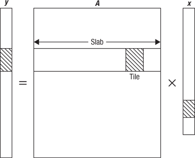
The global view of the tiled matrix representation is that the full matrix (complete with all of the zero elements) is partitioned into large rows of tiles (called slabs) whose width spans the entire width of the matrix and whose height corresponds to a contiguous subset of the output vector. Each tile in this row of tiles corresponds to an appropriately large contiguous subset of the input vector. Figure 22.2 shows a full matrix being multiplied by an input vector to compute an output vector. The hatched section of the matrix is a tile, within a row of tiles. The contiguous hatched areas of the input and output vectors are those that are used in conjunction with this matrix tile.
Figure 22.2 A tile in a matrix and its relationship with input and output vectors
The process of packetizing the slab proceeds in one of two ways, both involving a logical partition into strips of 16 matrix rows each. For devices that benefit from having local copies of contiguous sections of input vector, the strips are contained within the tiles. For devices that only access input data directly from global memory, the strips span the entire slab. Each strip is the source for a series of 16-element packets, where each of these 16 elements is sourced from a different row of the strip.
These packets also contain index and control information. If the elements are single precision, the packet is 128 bytes long. If the elements are double precision, the packet is 192 bytes long.
Each packet contains the following:
• A word specifying the global offset into the index vector of the hatched region affected by the tile containing the packet (which corresponds to the column in the full matrix where this tile begins)
• The input offset for the next tile, to allow devices whose memory subsystems can operate in parallel with the computations to preload the next section of the input vector
• A count of how many packets remain in this tile, to allow the kernels to control their loop structures
• The offset into the output vector, relative to the global offset specified in the second word of the header block above elements (which, again, corresponds to a row offset within the matrix) where the 16 output values are to be accumulated into 16 consecutive vectors
• Four words (16 bytes) of pad to ensure that the indices that follow are on a 32-byte boundary, and the floating-point data following those is on a 64-byte boundary (this is important for all architectures)
• Sixteen 2-byte input indices, relative to the input offset, one for each element of the packet
• Sixteen floating-point elements (single or double precision), which are actual non-zero data from the full matrix
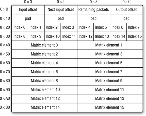
The organization of the packet is as shown in Figures 22.3 and 22.4 (each line comprises 16 bytes of this packet format).
Figure 22.3 Format of a single-precision 128-byte packet
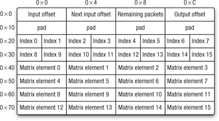
Figure 22.4 Format of a double-precision 192-byte packet
Header Structure
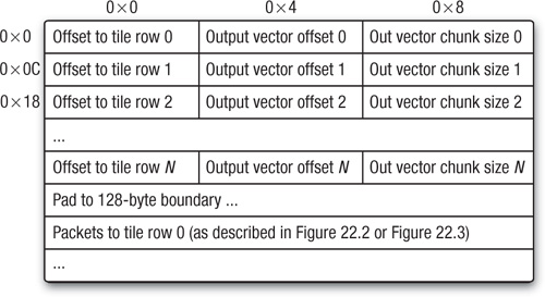
The overall structure of this tiled and packetized sparse matrix starts with a header block. The header block contains three 4-byte words of data per tile row consisting of the following:
• The offset into the tiled matrix memory structure where this slab’s packets begin
• The offset into the output vector where this slab’s computational results should be written (which corresponds to a row number in the full matrix)
• The number of contiguous elements of the output vector computed by this slab (corresponding to the number of contiguous rows of the full matrix that are represented by this slab)
The format is as shown in Figure 22.5.
Figure 22.5 Format of the header block of a tiled and packetized sparse matrix
Tiled and Packetized Sparse Matrix Design Considerations
The pad to 128-byte boundary is included for the benefit of all architectures, because data packets that reside on 64-byte boundaries perform better on GPUs and on cache-enabled CPUs, and because we always read even-sized groups of packets, they also improve the speed of async_work_group_copy commands in Cell/B.E. Accelerator devices, which work best with 128-byte alignment.
The configuration of 16 elements and 16 indices is chosen to correspond with common cache line sizes, common team sizes on GPUs, and the minimum size for moving memory parcels in some architectures. The load store kernel contains logic to enable different processing for GPU and CPU architectures.
The data is organized into the packets to guarantee that the elements in the packet correspond to consecutive rows of the matrix, so that a single block write of computed results serves to update the output vector that is the target of the computations involving this matrix, also eliminating the need to have 16 separate row indices, but rather a single index (the output offset shown in Figures 22.2 and 22.3). Essentially, this means that one must gather elements from the input vector to work with this packet, but there is no scatter operation after computations. Instead, we need only execute a single 64-byte or 128-byte read/modify/write for each packet to update the output.
Optional Team Information
In the case where the local work-group size is large (when use of GPUs is contemplated), this sample is further optimized through the inclusion of data specifying for each compute unit within the GPU where its first packet is and how many packets are to be processed. One or more initial packets in each slab is repurposed to contain this data. Each team needs to know the offset and length for its section of the slab.
For the purposes of this sample, two 2-byte quantities suffice to hold the offset and length, although these could be expanded to 4 bytes each if the matrices are large enough to require it. Thus, work-group sizes up to 512 can be accommodated with a single repurposed packet (512/16 is 32, and 4 bytes of data for each team adds up to 128 bytes). When the work-group size exceeds 512, more initial packets are used to contain the data.
Tested Hardware Devices and Results
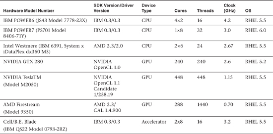
This implementation was run and verified on six hardware platforms, described in Table 22.1, all running OpenCL version 1.1, except for the GTX 280.
Table 22.1 Hardware Device Information
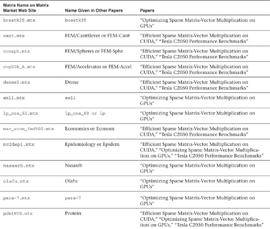
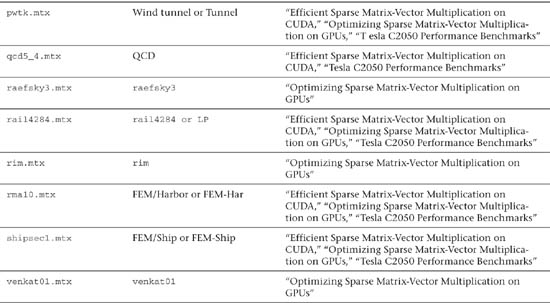
This sample was run on 22 different matrices. One of these was created as a sample (sample.mtx), and the other 21 were downloaded from the University of Florida Matrix Market Web site. Table 22.2 lists these 21 matrices, with references detailing which matrices were found in which of three previous papers on this subject.
Table 22.2 Sparse Matrix Description
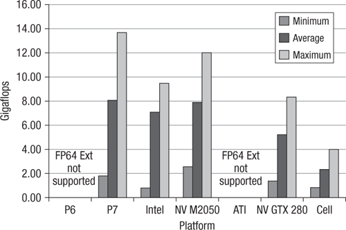
For brevity, the two performance charts in Figures 22.6 and 22.7 listing the minimum, maximum, and average performance over all 22 matrices are provided for each hardware device tested. Results for both double and single precision are presented, to the extent that the devices support them.
Figure 22.6 Single-precision SpMV performance across 22 matrices on seven platforms
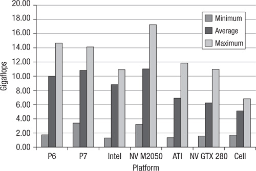
Figure 22.7 Double-precision SpMV performance across 22 matrices on five platforms
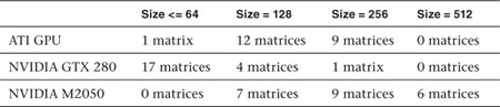
For each matrix, when running on GPUs, various local work-group sizes were investigated to determine the optimum size. Over the 22 matrices, the GPUs delivered optimal performance according to the histogram in Table 22.3.
Table 22.3 Optimal Performance Histogram for Various Matrix Sizes
It is important to mention the use or non-use of OpenCL image objects in GPUs at this point. Not all OpenCL implementations support access to image objects, so (for portability) this sample is not written to try to use image objects. On GPUs this decision precludes the use of texture memory and texture caches. Because the algorithm is memory-bound, this choice has performance implications, relative to implementations that exploit image objects. Here are some results quoted in two previous SpMV papers. The results in the first bullet point involve the use of texture memory, and the results in the second bullet point do not. Also, please note that the first bullet point compares results on an NVIDIA M2050, and the second compares results on an NVIDIA GeForce GTX 280.
• The two recommended methods listed for processing single precision in “Efficient Sparse Matrix-Vector Multiplication on CUDA” are hybrid and packet. For some matrices, hybrid is fastest, and for others, packet is fastest. Taking the average of these two methods across the 12 matrices that “Tesla C2050 Performance Benchmarks” shares in common with this chapter, the min/avg/max statistics for this CUDA/texture memory implementation are 7.0/16.2/23.2. This sample’s results over the same 12 matrices are 3.0/11.0/17.2.
• The two recommended methods listed for processing single-precision SpMV without cache (meaning without texture memory) in “Optimizing Sparse Matrix-Vector Multiplication on GPUs” are thread mapping and aligned access. In all cases listed, aligned access beats thread mapping. Across the 15 matrices this paper shares with this chapter, the min/avg/max statistics for this CUDA implementation are 0.3/6.1/9.75. This sample’s results over the same 15 matrices are 2.0/6.3/11.0.
Listing 22.1 describes the kernels that implement the sparse matrix-vector multiplication. The full source (kernels and host source code) for the histogram is provided in the Chapter_22/spmv directory of the book’s source code examples.
Listing 22.1 Sparse Matrix-Vector Multiplication OpenCL Kernels
/******************************************************************/
/* */
/* Licensed Materials - Property of IBM */
/* */
/* */
/* (C) Copyright IBM Corp. 2010 */
/* All Rights Reserved */
/* */
/* US Government Users Restricted Rights - Use, duplication or */
/* disclosure restricted by GSA ADP Schedule Contract with IBM */
/* Corp. */
/* */
/******************************************************************/
/* ============================================================== */
/* */
/* The "matbuffer" buffer contains the tiled matrix. */
/* The data in this tiled matrix is organized into "rows of */
/* tiles" which are called "slabs." */
/* The first section of this buffer contains three words of */
/* "header information" for each slab of the matrix. Each */
/* instantiation of the kernel is indexed by get_global_id(0) */
/* which matches the number of the slab. The three header words */
/* for each slab are: */
/* "offset": the offset into the buffer where the slab's */
/* data begins */
/* "outindex": the index into the output vector where this */
/* slab's output is to begin */
/* "outspan": the number of elements of the output vector */
/* which this slab is responsible for */
/* */
/* The actual data in the slab is organized into 16-element */
/* "packets" of length 128 bytes */
/* (see the definition of the "packet" struct below). */
/* Each packet contains four "control words" used by the kernels, */
/* 16 2-byte indices into the input array, and 16 */
/* floating-point values from the matrix. */
/* */
/* The four "control words" are: */
/* 0: base offset into the input vector for this packet */
/* 1: base offset into the input vector for a FUTURE packet */
/* (useful for double buffering) */
/* 2: the number of packets remaining in this slab */
/* 3: the offset (relative to the second header word) into the */
/* output vector for this packet */
/* */
/* These four words are followed by four words of pad, reserved */
/* for future use. Next come 16 short integers, containing */
/* offsets into the input vector. Next come 16 floating-point */
/* values, containing the actual matrix data. */
/* */
/* Specific output offsets for each value are not needed, because */
/* the packets are created in a special format: each value is */
/* intended to update the output vector element subsequent to */
/* that of the previous value. So, if a packet is targeted to */
/* location 512 of the output vector, then the 16 values in the */
/* packet will be updating locations 512 through 527 of the */
/* output vector respectively, and in order. This adds to the */
/* complexity of the code which creates these packets but results */
/* in significant performance payoffs, when performing the */
/* multiplications. */
/* */
/* It's frequently the case that there is empty data in these */
/* packets because of this construction. This data is carefully */
/* set up so that when we are dealing with local buffers, the */
/* garbage calculations go into an area which never gets written */
/* back to main memory. In the case where global memory is */
/* accessed directly, the "matrix data" in the empty values is */
/* set to zero, so that regardless of what the input is, the */
/* output is unaffected. */
/* */
/* ============================================================== */
/* These two structures are defined both in spmv.c and spmv.cl */
/* (using different variable types). */
/* If you change something here, change it in the other file as */
/* well. */
typedef struct _slab_header {
uint offset;
uint outindex;
uint outspan;
} slab_header;
typedef struct _packet {
uint seg_input_offset;
uint future_seg_input_offset;
uint npackets_remaining;
uint seg_output_offset;
uint pad1;
uint pad2;
uint pad3;
uint pad4;
ushort input_offset_short[16];
union {
float8 matdataV8[2];
float matdata[16];
} uf;
} packet;
/* ============================================================== */
/* Kernel using basic load/store mechanisms and local vars. This */
/* version is optimized for the GPU and CPU devices */
/* ============================================================== */
__kernel void tiled_spmv_kernel_LS(
__global float *input,
__global float *output,
__global uint *matbuffer,
uint column_span,
uint slabspace,
uint team_size,
uint num_header_packets,
__local float *outputspace)
{
uint i, gunit, lunit, start, span, npackets, teamnum, n_teams,
outindex, outspan;
__global slab_header *headptr;
__global float *work_input;
__global packet *gsegptr;
__global packet *gsegptr_stop;
__global float *outptr;
__local float *outptr16;
/* The local work-group is interpreted as a set of "teams," */
/* each consisting of 1 or 16 work units. This construction */
/* is frequently very useful on the GPU device. */
headptr = ((__global slab_header *) matbuffer) +
get_global_id(1);
outspan = headptr->outspan;
outindex = headptr->outindex;
n_teams = get_local_size(0)/team_size; /* number of teams */
gunit = get_local_id(0);
teamnum = gunit/team_size; /* which team is this? */
start = get_global_id(0); /* where in the packets is my */
/* "first word"? */
span = get_global_size(0); /* what stride shall I use when */
/* clearing or transmitting output */
/* buffers? */
/* Zero out the output buffer */
/* Each team has its own separate output buffer. */
/* At the end, these are accumulated. */
for (i = start; i < slabspace; i += span) {
#ifdef DOUBLE
outputspace[i] = 0.0;
#else
outputspace[i] = 0.0f;
#endif
}
barrier(CLK_LOCAL_MEM_FENCE);
/* Pointer to the start of the packets. */
gsegptr = &(((__global packet *) matbuffer)[headptr->offset]);
/* Pointer to pertinent area of output vector. */
outptr = &output[outindex];
/* We have two clauses here. The first is optimized for the */
/* GPU device, and the second is optimized for the CPU */
/* device. The distinction is that in the GPU device the */
/* memory access pattern for each work unit is strided, and */
/* in the CPU device, the memory access pattern is contiguous.*/
/* Virtually all processing happens in the selected clause */
/* below. */
if (team_size == 16) {
lunit = gunit % team_size; /* Which work unit within the */
/* team am I? */
__global uint *first_team_offset;
first_team_offset = (__global uint *) gsegptr;
int temp_offset, temp_packetcount;
temp_offset = first_team_offset[teamnum] / 65536;
temp_packetcount = first_team_offset[teamnum] % 65536;
gsegptr += num_header_packets + temp_offset;
for (i=0; i<temp_packetcount; ++i) {
outptr16 = &outputspace[gsegptr->seg_output_offset];
work_input = &input[gsegptr->seg_input_offset];
outptr16[lunit] += gsegptr->uf.matdata[lunit] *
work_input[gsegptr->input_offset_short[lunit]];
++gsegptr;
}
}
else { /* team_size is 1, and this work unit needs to do */
/* all 16 elements in the packet */
/* skip over team_offset data */
gsegptr += num_header_packets;
/* Number of packets to be processed. */
npackets = gsegptr->npackets_remaining;
int stopdex = ((teamnum + 1) * npackets) / n_teams;
int startdex = ((teamnum ) * npackets) / n_teams;
gsegptr_stop = &gsegptr[stopdex];
gsegptr = &gsegptr[startdex];
while (gsegptr < gsegptr_stop) {
outptr16 = &outputspace[gsegptr->seg_output_offset];
work_input = &input[gsegptr->seg_input_offset];
for (lunit=0; lunit<16; ++lunit) {
outptr16[lunit] += gsegptr->uf.matdata[lunit] *
work_input[gsegptr->input_offset_short[lunit]];
}
++gsegptr;
}
}
barrier(CLK_LOCAL_MEM_FENCE);
/* Now that processing is done, it's time to write out */
/* the final results for this slab. */
for (i=start; i<outspan; i+=span) {
outptr[i] = outputspace[i];
}
}
/* =========================================================== */
/* Kernel using "async_work_group_copy". This version is */
/* optimized for the ACCELERATOR device */
/* =========================================================== */
/* =========================================================== */
/* Grab a pile of input vector data into local storage */
/* "_inputspace_index" is the offset into the local space. */
/* "_input_offset" is the offset into the global input vector. */
/* =========================================================== */
#define GET_INPUT(_inputspace_index, _input_offset) {
eventI[_inputspace_index] = async_work_group_copy(
(__local float8 *)&inputspace[column_span * _inputspace_index],
(const __global float8 *) &input[_input_offset],
(size_t) (column_span>>3),
(event_t) 0);
}
/* ========================================================= */
/* Grab a pile of matrix packets into local storage */
/* "_lsegspace_index" specifies the correct offset. */
/* ========================================================= */
#define GET_PACKET(_lsegspace_index) {
eventS[lsegspace_tag] = async_work_group_copy(
(__local uchar16 *) &lsegspace[(_lsegspace_index)],
(const __global uchar16 *) &gsegptr[gseg_index],
(size_t) ((sizeof(packet)/16)*(segcachesize/2)),
(event_t) 0);
gseg_index += (segcachesize/2);
}
/* ========================================================= */
/* */
/* For a given packet of matrix data, residing in LOCAL */
/* memory, do the following: */
/* Snap a pointer to the beginning of the packet. */
/* If it's time, grab a new batch of input data. */
/* Snap pointers to the output and matrix float data. */
/* Spend 16 lines performing the scalar computations. */
/* Perform two 8-way SIMD FMA operations. */
/* Update the index to the next packet. */
/* */
/* ========================================================= */
#define PROCESS_LOCAL_PACKET {
float8 inV[2];
lsegptr = (__local struct _packet *)
&lsegspace[lsegspace_index];
if (lsegptr->seg_input_offset != curr_input_offset) {
curr_input_offset = lsegptr->seg_input_offset;
next_input_offset = lsegptr->future_seg_input_offset;
GET_INPUT(inputspace_index, next_input_offset)
inputspace_index = 1 - inputspace_index;
wait_group_events(1, &eventI[inputspace_index]);
}
work_input = &inputspace[column_span * inputspace_index];
outputspaceV8 = (__local float8 *)
&outputspace[lsegptr->seg_output_offset];
inV[0].s0 = work_input[lsegptr->input_offset_short[ 0]];
inV[0].s1 = work_input[lsegptr->input_offset_short[ 1]];
inV[0].s2 = work_input[lsegptr->input_offset_short[ 2]];
inV[0].s3 = work_input[lsegptr->input_offset_short[ 3]];
inV[0].s4 = work_input[lsegptr->input_offset_short[ 4]];
inV[0].s5 = work_input[lsegptr->input_offset_short[ 5]];
inV[0].s6 = work_input[lsegptr->input_offset_short[ 6]];
inV[0].s7 = work_input[lsegptr->input_offset_short[ 7]];
inV[1].s0 = work_input[lsegptr->input_offset_short[ 8]];
inV[1].s1 = work_input[lsegptr->input_offset_short[ 9]];
inV[1].s2 = work_input[lsegptr->input_offset_short[10]];
inV[1].s3 = work_input[lsegptr->input_offset_short[11]];
inV[1].s4 = work_input[lsegptr->input_offset_short[12]];
inV[1].s5 = work_input[lsegptr->input_offset_short[13]];
inV[1].s6 = work_input[lsegptr->input_offset_short[14]];
inV[1].s7 = work_input[lsegptr->input_offset_short[15]];
outputspaceV8[0] = fma(lsegptr->uf.matdataV8[0], inV[0],
outputspaceV8[0]);
outputspaceV8[1] = fma(lsegptr->uf.matdataV8[1], inV[1],
outputspaceV8[1]);
++lsegspace_index;
}
__kernel __attribute__ ((reqd_work_group_size(1, 1, 1)))
void tiled_spmv_kernel_AWGC(
__global float *input, /* pointer to input memory object */
__global float *output,/* pointer to output memory object */
__global uint *matbuffer, /* pointer to tiled matrix */
/* memory object in global */
/* memory */
uint column_span, /* size of fixed chunks of the input */
/* vector */
uint slabspace, /* size of the variable chunk of output */
/* vector to be computed */
uint segcachesize, /* number of tiled matrix packets */
/* which fit in "outputspace" */
uint num_header_packets,
__local float *inputspace, /* local buffer to hold staged */
/* input vector data */
__local float *outputspace, /* local buffer to hold */
/* computed output, to be written */
/* out at the end */
__local packet *lsegspace) /* local buffer to hold staged */
/* tiled matrix packet data */
{
__global slab_header *headptr;
__local float *work_input;
__local float8 *outputspaceV8;
int i, tempmax;
event_t eventS[2], eventI[2], eventO;
int temp = segcachesize/2;
int half_scs = 0;
while (temp) {
++half_scs;
temp >>= 1;
}
/* This is a global packet pointer, indexing into the global */
/* memory object containing the tiled matrix */
__global packet *gsegptr;
/* This is a local packet pointer, indexing into the local */
/* storage for our tiled matrix */
__local packet *lsegptr;
headptr = ((__global slab_header *) matbuffer)
+ get_global_id(0);
gsegptr = &(((__global packet *) matbuffer)[headptr->offset]);
gsegptr += num_header_packets; /* skip over team_offset data */
lsegptr = &lsegspace[0];
int gseg_index = 0; /* index into global memory of the */
/* packets for this slab */
int inputspace_index = 0; /* offset index into the local */
/* space for the input */
int lsegspace_index = 0; /* offset index into the local */
/* space for the tiled matrix */
int lsegspace_tag = 0; /* tag used to manage events */
/* regarding local packets */
GET_PACKET(0)
wait_group_events(1, &eventS[0]);
/* how many packets are to be processed in this slab? */
uint npackets = lsegptr->npackets_remaining;
if (npackets == 0) return;
GET_PACKET(segcachesize/2)
tempmax = (segcachesize < npackets) ? segcachesize : npackets;
for (i=0; i<slabspace; ++i) {
outputspace[i] = 0.0f; /* zero out the output buffer */
}
uint curr_input_offset = lsegptr->seg_input_offset;
uint next_input_offset = lsegptr->future_seg_input_offset;
GET_INPUT(0, curr_input_offset) /* Load the first two parcels */
GET_INPUT(1, next_input_offset) /* of local input vector data */
/* and wait on the first one. */
wait_group_events(1, &eventI[inputspace_index]);
/* this first loop handles the bulk of the work with */
/* minimal if-tests, segcachesize/2 packets at a time */
while (npackets > tempmax) {
for (i=0; i<segcachesize/2; ++i) {
PROCESS_LOCAL_PACKET
}
/* load next batch of packets, using double buffering */
lsegspace_index &= (segcachesize-1);
lsegspace_tag = (lsegspace_index ==
(segcachesize/2)) ? 1 : 0;
npackets -= segcachesize/2;
GET_PACKET((segcachesize/2)-lsegspace_index);
wait_group_events(1, &eventS[lsegspace_tag]);
}
/* this second loop handles the remaining packets, one packet */
/* at a time */
while (npackets) {
PROCESS_LOCAL_PACKET
lsegspace_index &= (segcachesize-1);
lsegspace_tag = (lsegspace_index ==
(segcachesize/2)) ? 1 : 0;
--npackets;
if ((lsegspace_index & ((segcachesize/2)-1)) == 0) {
if (npackets > segcachesize/2) {
GET_PACKET((segcachesize/2)-lsegspace_index);
}
if (npackets > 0) {
wait_group_events(1, &eventS[lsegspace_tag]);
}
}
}
/* Now that processing is done, it's time to write out the */
/* final results for this slab. */
eventO = async_work_group_copy(
(__global float *) &output[headptr->outindex],
(__const local float *) outputspace,
(size_t) (headptr->outspan),
(event_t) 0);
wait_group_events(1, &eventO);
wait_group_events(1, &eventI[1-inputspace_index]);
wait_group_events(2, eventS);
}
Additional Areas of Optimization
The number of packets from any slice must be equal to the maximum number of non-zero elements found in any of its rows. Because the other rows will typically have fewer elements, some packets will be loaded with null elements (whose matrix floating-point value is zero). This “reduction in packet density” has the effect of reducing performance, and the correlation is quite high. In fact, across the 22 matrices studied, and across four hardware platforms, the averaged statistical correlation between gigaflops and packet density was ρ = 0.8733.
An optimization for this packet density inefficiency is to permute the rows within each slab according to their non-zero element count. The algorithmically complete permutation would be a full sort, but simpler (and faster) heuristics might suffice. This would require adding a permutation array to each slab in the data structure. The kernels would read in that permutation array and use it to scatter the output data when they are completely finished with the slab, which won’t add significantly to the total compute time. This improvement guarantees that we get roughly the same gigaflop performance from all matrices, no matter how ill formed they are.